Datasaurus
Aurelien Ginolhac
2021-07-22
This guided practical will demonstrate that the tidyverse allows to compute summary statistics and visualize datasets efficiently. This dataset is already stored in a tidy tibble, cleaning steps will come in future practicals.
Those kind of questions are optional
datasauRus package
- check if you have the package
datasauRusinstalled
library(datasauRus)- should return nothing. If
there is no package called ‘datasauRus’appears, it means that the package needs to be installed. Use this:
install.packages("datasauRus")Explore the dataset
Since we are dealing with a tibble, we can just type
datasaurus_dozenonly the first 10 rows are displayed.
| dataset | x | y |
|---|---|---|
| dino | 55.3846 | 97.1795 |
| dino | 51.5385 | 96.0256 |
| dino | 46.1538 | 94.4872 |
| dino | 42.8205 | 91.4103 |
| dino | 40.7692 | 88.3333 |
| dino | 38.7179 | 84.8718 |
| dino | 35.6410 | 79.8718 |
| dino | 33.0769 | 77.5641 |
| dino | 28.9744 | 74.4872 |
| dino | 26.1538 | 71.4103 |
What are the dimensions of this dataset? Rows and columns?
- base version, using either
dim(),ncol()andnrow()
# dim() returns the dimensions of the data frame, i.e number of rows and columns
dim(datasaurus_dozen)
## [1] 1846 3# ncol() only number of columns
ncol(datasaurus_dozen)## [1] 3# nrow() only number of rows
nrow(datasaurus_dozen)## [1] 1846- tidyverse version
nothing to be done, a
tibble display its dimensions, starting by a comment (‘#’ character)
Assign the datasaurus_dozen to the ds_dozen name This aims at populating the Global Environment
ds_dozen <- datasaurus_dozenUsing Rstudio, those dimensions are now also reported within the interface, where?
in the Environment panel -> Global Environment
How many datasets are present?
- base version
Tip
you want to count the number of unique elements in the column dataset. The function length() returns the length of a vector, such as the unique elements
unique(ds_dozen$dataset) %>% length()## [1] 13- tidyverse version
# n_distinct counts the unique elements in a given vector.
# we use summarise to return only the desired column named n here.
summarise(ds_dozen, n = n_distinct(dataset))
## # A tibble: 1 x 1
## n
## <int>
## 1 13- even better way, compute and display the number of lines per
dataset
Tip
the function
count in dplyr does the group_by() by the specified column + summarise(n = n()) which returns the number of observation per defined group.
count(ds_dozen, dataset)## # A tibble: 13 x 2
## dataset n
## <chr> <int>
## 1 away 142
## 2 bullseye 142
## 3 circle 142
## 4 dino 142
## 5 dots 142
## 6 h_lines 142
## 7 high_lines 142
## 8 slant_down 142
## 9 slant_up 142
## 10 star 142
## 11 v_lines 142
## 12 wide_lines 142
## 13 x_shape 142Check summary statistics per dataset
Compute the mean of the x & y column. For this, you need to group_by() the appropriate column and then summarise()
Tip
in
summarise() you can define as many new columns as you wish. No need to call it for every single variable.
ds_dozen %>%
  group_by(dataset) %>%
  summarise(mean_x = mean(x),
mean_y = mean(y))| dataset | mean_x | mean_y |
|---|---|---|
| away | 54.26610 | 47.83472 |
| bullseye | 54.26873 | 47.83082 |
| circle | 54.26732 | 47.83772 |
| dino | 54.26327 | 47.83225 |
| dots | 54.26030 | 47.83983 |
| h_lines | 54.26144 | 47.83025 |
| high_lines | 54.26881 | 47.83545 |
| slant_down | 54.26785 | 47.83590 |
| slant_up | 54.26588 | 47.83150 |
| star | 54.26734 | 47.83955 |
| v_lines | 54.26993 | 47.83699 |
| wide_lines | 54.26692 | 47.83160 |
| x_shape | 54.26015 | 47.83972 |
Compute both mean and standard deviation (sd) in one go using across()
ds_dozen %>%
  group_by(dataset) %>%
  # across works with first on which columns and second on what to perform on selection
  # 2 possibilities to select columns
  # summarise(across(where(is.double), list(mean = mean, sd = sd)))
summarise(across(c(x, y), list(mean = mean, sd = sd)))| dataset | x_mean | x_sd | y_mean | y_sd |
|---|---|---|---|---|
| away | 54.26610 | 16.76983 | 47.83472 | 26.93974 |
| bullseye | 54.26873 | 16.76924 | 47.83082 | 26.93573 |
| circle | 54.26732 | 16.76001 | 47.83772 | 26.93004 |
| dino | 54.26327 | 16.76514 | 47.83225 | 26.93540 |
| dots | 54.26030 | 16.76774 | 47.83983 | 26.93019 |
| h_lines | 54.26144 | 16.76590 | 47.83025 | 26.93988 |
| high_lines | 54.26881 | 16.76670 | 47.83545 | 26.94000 |
| slant_down | 54.26785 | 16.76676 | 47.83590 | 26.93610 |
| slant_up | 54.26588 | 16.76885 | 47.83150 | 26.93861 |
| star | 54.26734 | 16.76896 | 47.83955 | 26.93027 |
| v_lines | 54.26993 | 16.76996 | 47.83699 | 26.93768 |
| wide_lines | 54.26692 | 16.77000 | 47.83160 | 26.93790 |
| x_shape | 54.26015 | 16.76996 | 47.83972 | 26.93000 |
What can you conclude?
all mean and sd are the same for the 13 datasets
Plot the datasauRus
Plot the ds_dozen with ggplot such the aesthetics are aes(x = x, y = y)
with the geometry geom_point()
Tip
the
ggplot() and geom_point() functions must be linked with a + sign
ggplot(ds_dozen, aes(x = x, y = y)) +
  geom_point()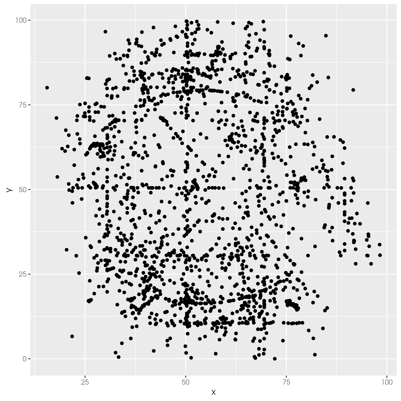
Reuse the above command, and now colored by the dataset column
ggplot(ds_dozen, aes(x = x, y = y, colour = dataset)) +
  geom_point()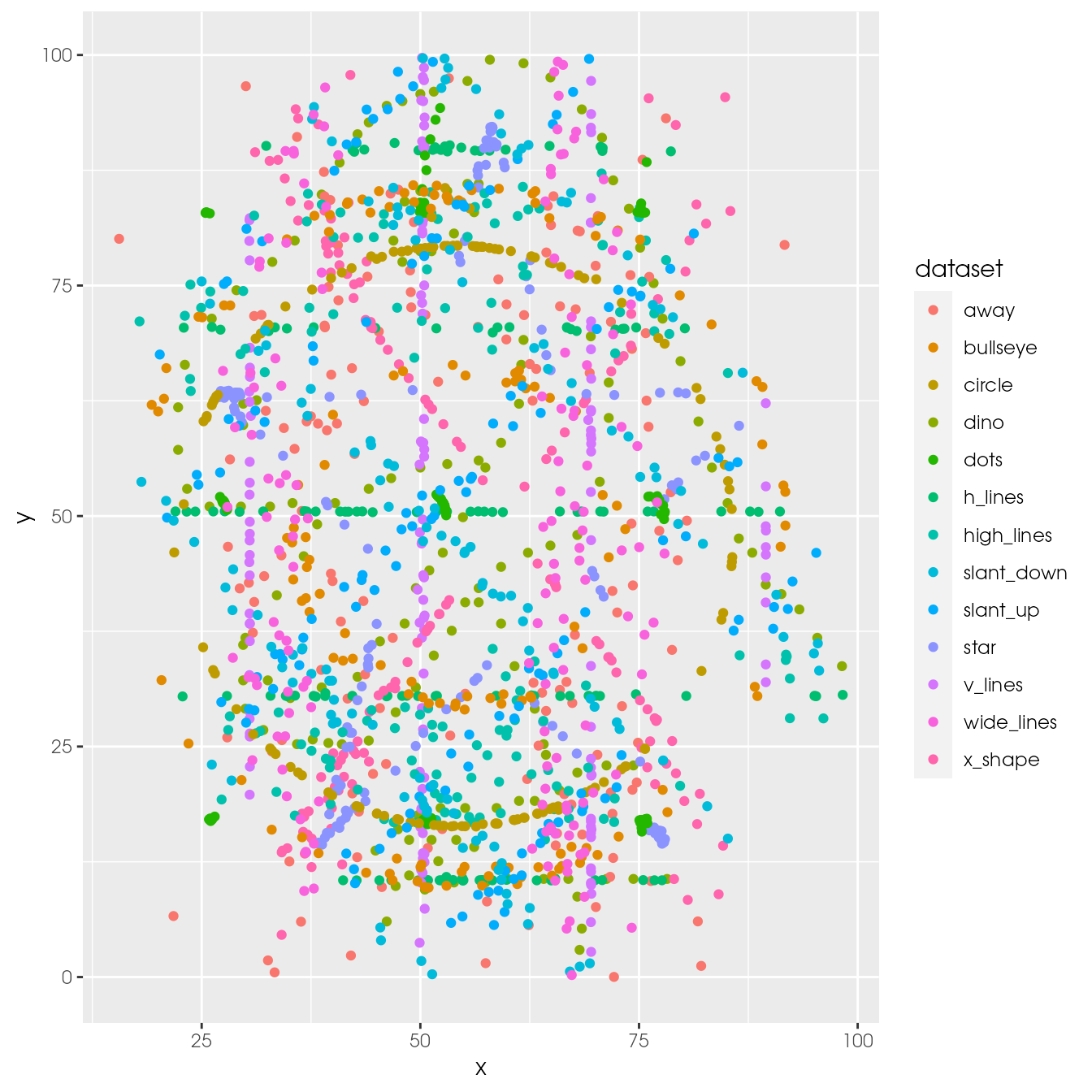
Too many datasets are displayed.
How can we plot only one at a time?
Tip
You can filter for one dataset upstream of plotting
ds_dozen %>%
  filter(dataset == "away") %>%
  ggplot(aes(x = x, y = y)) +
  geom_point()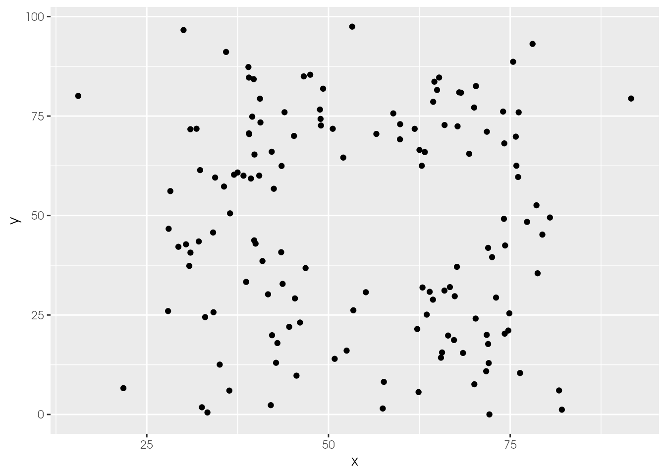
Adjust the filtering step to plot two datasets
Tip
R provides the inline instruction
%in% to test if there a match of the left operand in the right one (a vector most probably)
ds_dozen %>%
  filter(dataset %in% c("away", "dino")) %>%
  # alternative without %in% and using OR (|)
  #filter(dataset == "away" | dataset == "dino") %>%
  ggplot(aes(x = x, y = y, colour = dataset)) +
  geom_point()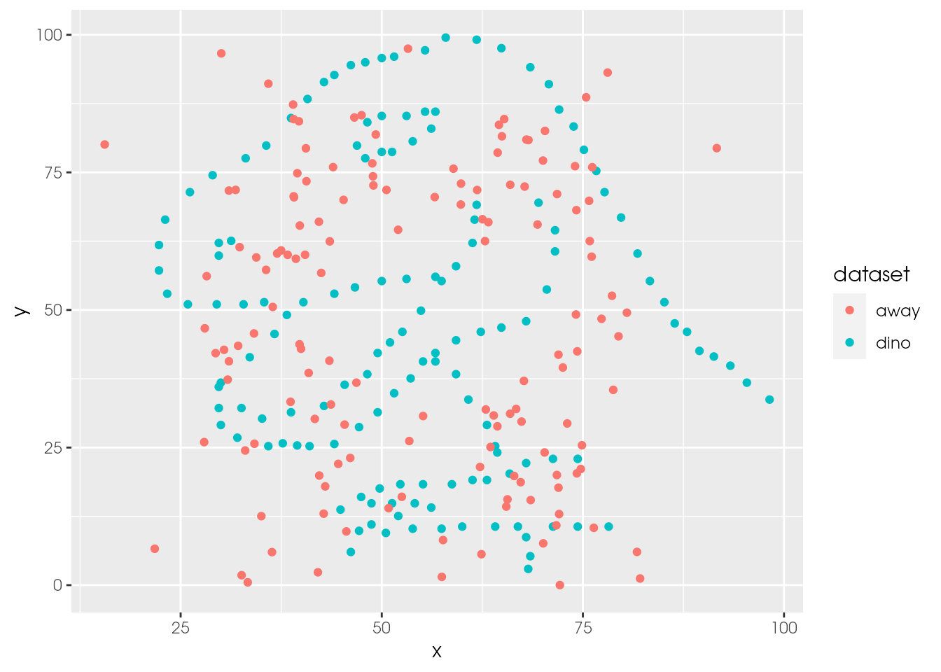
Expand now by getting one dataset per facet
ds_dozen %>%
  filter(dataset %in% c("away", "dino")) %>%
  ggplot(aes(x = x, y = y, colour = dataset)) +
  geom_point() +
  facet_wrap(~ dataset)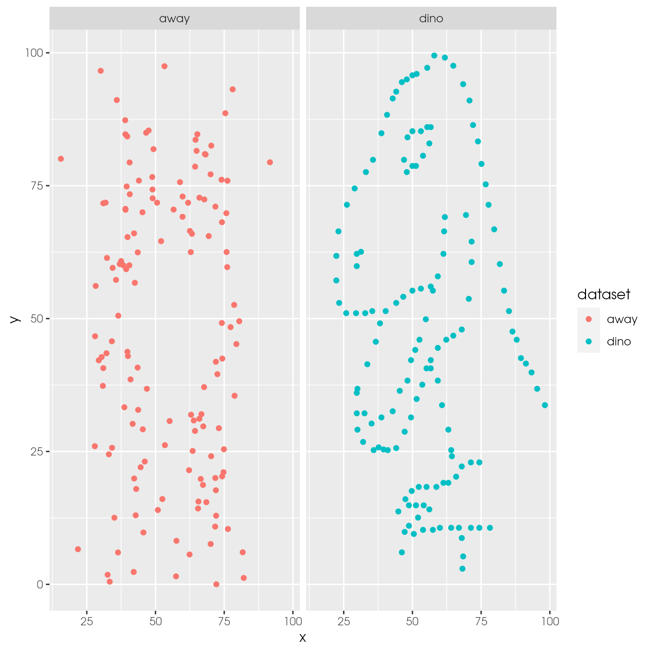
Remove the filtering step to facet all datasets
ds_dozen %>%
  ggplot(aes(x = x, y = y, colour = dataset)) +
  geom_point() +
  facet_wrap(~ dataset, ncol = 3)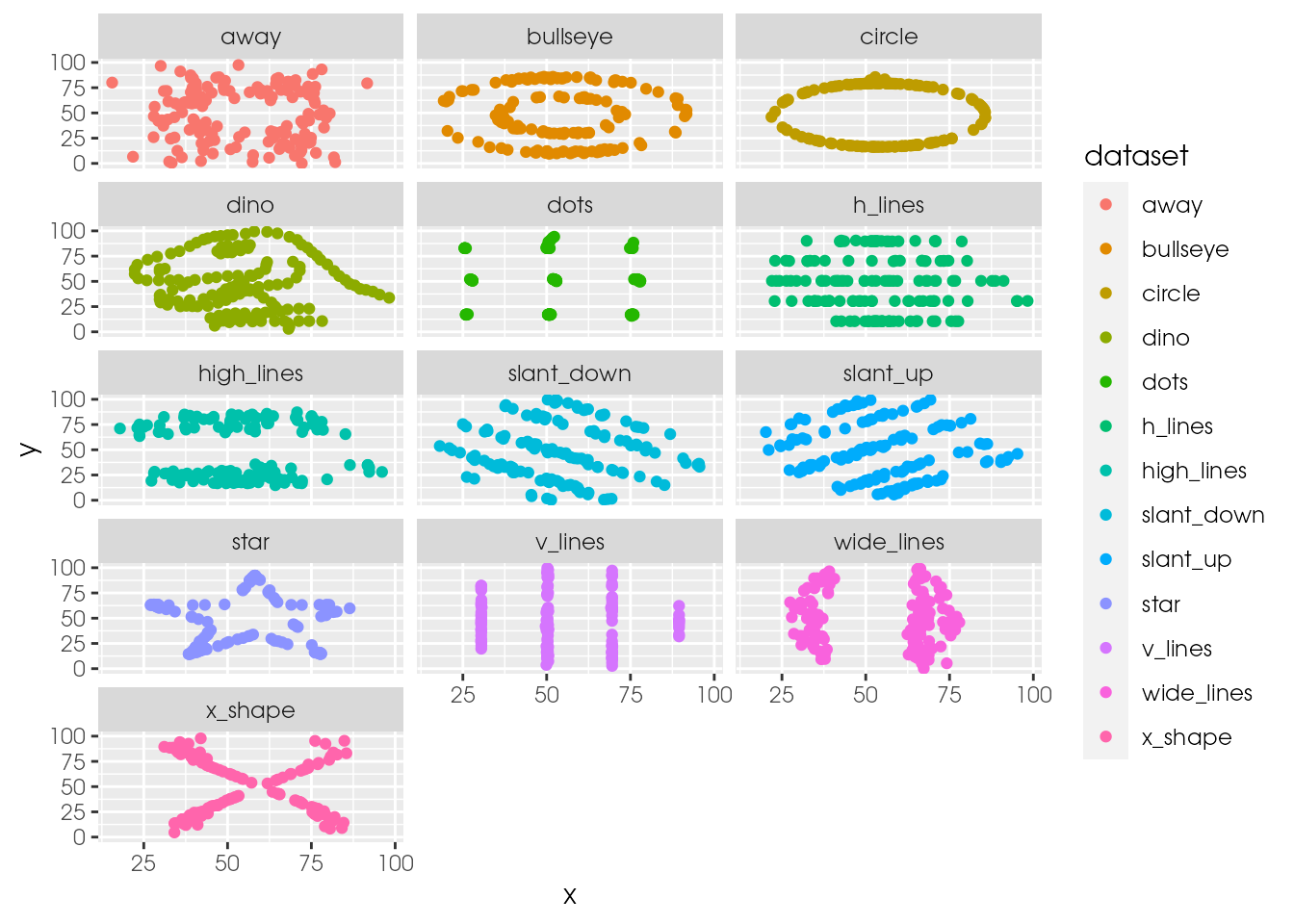
Tweak the theme and use the theme_void and remove the legend
ggplot(ds_dozen, aes(x = x, y = y, colour = dataset)) +
  geom_point() +
  theme_void() +
  theme(legend.position = "none") +
  facet_wrap(~ dataset, ncol = 3)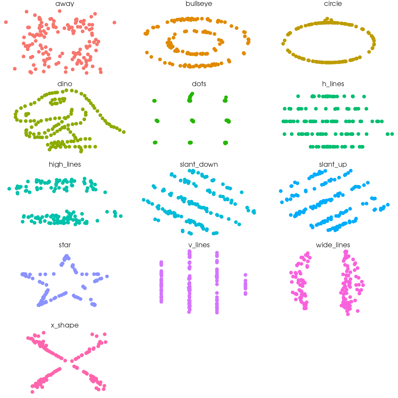
Are the datasets actually that similar?
No ;) We were fooled by the summary stats
Tip
the R package
gifski could be installed on your machine, makes the GIF creation faster. gifski is internally written in rust, and this language needs cargo to run. See this article to get it installed on your machine. First install rust before install the R package gifski. Please note, that the animate() step still takes ~ 3-5 minutes depending on your machine.
Install gganimate, its dependencies will be automatically installed.
install.packages("gganimate")Use the dataset variable to the transition_states() argument layer
library(gganimate)

ds_dozen %>%
  ggplot(aes(x = x, y = y)) +
  geom_point() +
  # transition will be made using the dataset column
  transition_states(dataset, transition_length = 5, state_length = 2) +
  # for a firework effect!
  shadow_wake(wake_length = 0.05) +
  labs(title = "dataset: {closest_state}") +
  theme_void(14) +
  theme(legend.position = "none") -> ds_anim
# more frames to slow down the animation
ds_gif <- animate(ds_anim, nframes = 500, fps = 10, renderer = gifski_renderer())
ds_gif
anim_save(title_frame = TRUE, "./img/ds.gif")
Visualize the tiny differences in means for both coordinates
- need to zoom tremendously to see differences. Accumulate all states to better see the motions.
ds_dozen %>%
  group_by(dataset) %>%
  summarise(across(c(x, y), list(mean = mean, sd = sd))) %>%
  ggplot(aes(x = x_mean, y = y_mean, colour = dataset)) +
  geom_point(size = 25, alpha = 0.6) +
  # zoom in like crazy
  coord_cartesian(xlim = c(54.25, 54.3), ylim = c(47.75, 47.9)) +
  # animate
  transition_states(dataset, transition_length = 5, state_length = 2) +
  # do not remove previous states to pile up dots
  shadow_mark() +
  labs(title = "dataset: {closest_state}") +
  theme_minimal(14) +
  theme(legend.position = "none") -> ds_mean_anim
ds_mean_gif <- animate(ds_mean_anim, nframes = 100, fps = 10)
ds_mean_gif
anim_save("img/ds_mean.gif")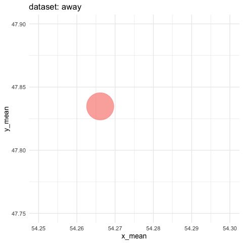
Conclusion
never trust summary statistics alone; always visualize your data | Alberto Cairo
Authors
- Alberto Cairo, (creator)
- Justin Matejka
- George Fitzmaurice
- Lucy McGowan
from this post