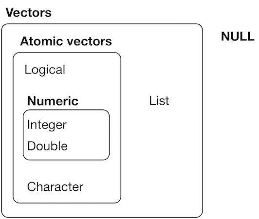
Introduction to the course

R base and the tidyverse

Roland Krause

Rworkshop

Tuesday, 6 February 2024

Good morning and welcome to Rworkshop!

What you can do now

Check for material at the main site

https://rworkshop.uni.lu

Install R, RStudio and packages
Check your install

GitHub account
- Mandatory for the practicals
- Clone the practical and start the setup. Check here for details.
Communicate
- Drink coffee or tea in room 2.150.

Introduction

30 March 2016

Dear all, I would like to organize a workshop for the LSRU and LCSB people who want to learn / improve their R skills. Starting from scratch a R course does not seem relevant neither effective. On the contrary, learning from concrete examples and focusing on modern packages should help.

from:aurelien.ginolhac@uni.lu

# from https://github.com/ANGSD/angsd/blob/master/R/jackKnife.R
Args<-function(l,args){
 if(! all(sapply(strsplit(l,"="),function(x)x[1])%in%names(args))){
  cat("Error -> ",l[!sapply(strsplit(l,"="),function(x)x[1])%in%names(args)]," is not a valid argument")
  q("no")
}

Overview

This 4-day-course provides an introduction to the tidyverse, a dialect.

Focusing on loading and cleaning data for exploratory visualizations
Speeding data manipulation is the mission of this course
This workshop is composed of 30 hours:

Lectures - Days 1 - 4

Available online ( / )
Live exercises included

Practicals - Days 1 - 3

Using your own laptop and Github classroom
Supplementary exercises if needed

Concluding practical

Required for ECTS

Bring your own data - Day 4

Apply what you just learnt to your own data

Instructors

Aurélien Ginolhac - Conception, design, tooling

Organization

ECTS

1 ECTS are awarded to PhD students

For submitting all practicals through github classroom.

Operational suggestions

Don’t be afraid to ask any question.
If you need help during the exercises, practicals or projects, stick a post-it note to your machine.
Lunch is from 12.30 to 13.30. We can go in a group but take your time as needed.

What is really?

is shorthand for “GNU R”:

An interactive programming language derived from S (J. Chambers, Bell Lab, 1976)
Appeared in 1995, created by Ross Ihaka and Robert Gentleman, University of Auckland, NZ
Focus on data analysis and plotting
is also shorthand for the ecosystem around this language
- Book authors
- Package developers
- Ordinary useRs

Learning to use will make you more efficient and facilitate the use of advanced data analysis tools

Why using ?

It’s free! and open-source
Easy to install / maintain
Multi-platform (Windows, macOS, GNU/Linux)
Can process big files and analyse huge amounts of data (db tools)
Integrated data visualization tools, even dynamic shiny
Fast, and even faster with C++ integration via Rcpp or cpp11.
Easy to get help, welcoming community
- huge community in the web
- stackoverflow with a lot of tags like r, ggplot2 etc.
- rbloggers
- R ladies

Learning R

The bad news is that when ever you learn a new skill you’re going to suck. It’s going to be frustrating. The good news is that is typical and happens to everyone and it is only temporary. You can’t go from knowing nothing to becoming an expert without going through a period of great frustration and great suckiness.

— Hadley Wickham

is hard to learn

base is complex, has a long history and many contributors

Why is hard to learn

Unhelpful help ?print
Generic methods print.data.frame
Too many commands colnames, names
Inconsistent names read.csv, load, readRDS
Un-strict syntax, was designed for interactive usage
Too many ways to select variables df$x, df$"x", df[,"x"], df[[1]]
[…] see r4stats’ post for the full list
The tidyverse curse

Navigating the balance between base and the tidyverse is a challenge to learn

— Robert A. Muenchen

Help pages

2 possibilities for manual pages.

?log
help(log)

Sadly, manpages are often unhelpful, vignettes or articles better described workflow.

In Rstudio, the help page can be viewed in the bottom right pane

The ambiguity [of the S language] is real and goes to a key objective: we wanted users to be able to begin in an interactive environment, where they did not consciously think of themselves as programming. Then as their needs became clearer and their sophistication increased, they should be able slide gradually into programming, when the language and system aspects would become more important.

— John Chambers, “Stages in the Evolution of S”

Tidyverse origin

Hadley Wickham

Hadley is Chief Scientist at Rstudio

Coined the tidyverse at userR meeting in 2016
Developed and maintains most of the core tidyverse packages

We think the tidyverse is better, especially for beginners. It is:

Relatively recent (both an issue and an advantage)
Becomes stable
Allows doing powerful things quickly
Unified
Consistent, one way to do things
Give strength to learn base R

Tidyverse, core packages

Role of tidyverse packages in the R community

Tidyverse features introduced to base

Construct		Base R	Version
Pipe	`%>%`	`\|>`	v4.1
Placeholder in pipe	`.`	`_`	v4.2
lambda	`~ .x`	`\(x)`	v4.1
`c(factor("a"), factor("b"))`	Is `[1] a b`	Was `[1] 1 1`	v4.1
Strings read as factors	`tibbles` and `readr`	Default	v4.0

- a refresher

Naming symbols for this course

Common symbols

= - equal

. - dot

, - comma

> - greater than

< - less than

~ - twiddle

* - star

- - hyphen

_ - underscore

Quotation and comments

" - double quotation marks

' - single quotation marks

` - backticks

# - hash

| - (vertical) bar

/ - (forward) slash

\ - backslash

Enclosures

() - parentheses

[]- (square) brackets

{} - (curly) braces

<> - chevrons

R-specific operators

<- - assignment (left)

-> - right assignment

%>% - (magrittr) pipe

|> - (base) pipe

Using `library()`, ensure function’ origin

With only base loaded

x <- 1:10
filter(x, rep(1, 3))

Time Series:
Start = 1 
End = 10 
Frequency = 1 
 [1] NA  6  9 12 15 18 21 24 27 NA

Conflict: 2 packages export same function

With the same name, the latest loaded wins

library(dplyr)
filter(x, rep(1, 3))

Error in UseMethod("filter"): no applicable method for 'filter' applied to an object of class "c('integer', 'numeric')"

Solution: use :: to call functions from a specific package

stats::filter(x, rep(1, 3))

Time Series:
Start = 1 
End = 10 
Frequency = 1 
 [1] NA  6  9 12 15 18 21 24 27 NA

Data types and structures

4 main types

Type	Example
numeric	`integer` (`2`), `double` (`2.34`)
character (strings)	`"tidyverse!"`
boolean	`TRUE` / `FALSE` (`T`/`F` not protected)
complex	`2+0i`

Missing data and special cases

NA   # not available, missing data
NA_real_
NA_integer_
NA_character_
NA_complex_
NULL # empty
-Inf/Inf # infinite values
NaN # Not a Number

2L

[1] 2

typeof(2L)

[1] "integer"

2.34

[1] 2.34

typeof(2.34)

[1] "double"

"tidyverse!"

[1] "tidyverse!"

TRUE

[1] TRUE

2+0i

[1] 2+0i

Structures

Vectors

c() is the function for concatenate

[1] 4

c(43, 5.6, 2.90)

[1] 43.0  5.6  2.9

Factors

convert strings to factors, levels is the dictionary

factor(c("AA", "BB", "AA", "CC"))

[1] AA BB AA CC
Levels: AA BB CC

Lists

Can contain any other data type.

list(f = factor(c("AA", "AA")),
     v = c(43, 5.6, 2.90),
     s = 4L)

$f
[1] AA AA
Levels: AA

$v
[1] 43.0  5.6  2.9

$s
[1] 4

Data frames are special lists

`data.frame`

same as list but where all objects must have the same length

data.frame(
  f = factor(c("AA", "AA", "BB")),
  v = c(43, 5.6, 2.90),
  s = rep(4, 3))

   f    v s
1 AA 43.0 4
2 AA  5.6 4
3 BB  2.9 4

Example, missing one element in `v`

data.frame(
  f = factor(c("AA", "AA", "BB")),
  v = c(43, 5.6),
  s = rep(4, 3))

Error in data.frame(f = factor(c("AA", "AA", "BB")), v = c(43, 5.6), s = rep(4, : arguments imply differing number of rows: 3, 2

Concatenate atomic elements

Collection of simple things

Things are the smallest elements: atomic
Must be of same mode: automatic coercion
Indexed, from 1 to length(vector)
Created with the c() function

c(2, TRUE, "a string")

[1] "2"        "TRUE"     "a string"

Manual coercion

as.character(c(2, TRUE, "a string"))

[1] "2"        "TRUE"     "a string"

as.double(c(2, TRUE, "a string"))

[1]  2 NA NA

as.double(c(2, 2.456, "a string"))

[1] 2.000 2.456    NA

Assignment

Operator is <-, associate a name to an object

right version -> is a valid alias

my_vec <- c(3, 4, 1:3)
my_vec

[1] 3 4 1 2 3

Say: the vector gets assigned the name my_vec

Tip

Rstudio has the built-in shortcut Alt+- for <-

Rationale

If you don’t assigned a name to a created object it is only temporary. Assigning allows to save and re-use the object for a downstream step.

Binding names to values: an object has no name

In #rstats, it's surprisingly important to realise that names have objects; objects don't have names pic.twitter.com/bEMO1YVZX0
— Hadley Wickham (@hadleywickham) May 16, 2016

Vector is bind to the name `x`

x <- 1:3

Same vector is also bind to the name `y`

y <- x

Hierarchy

is.vector(c("a", "c"))

[1] TRUE

is.vector(list(a = 1))

[1] TRUE

is.atomic(list(a = 1))

[1] FALSE

is.data.frame(list(a = 1))

[1] FALSE

Subsetting vectors

Caution

Unlike python or Perl, vectors use 1-based index!!

Generate `integer` sequence

3:10

[1]  3  4  5  6  7  8  9 10

Subset elements

Select elements from position 3 to 10:

LETTERS[3:10]

[1] "C" "D" "E" "F" "G" "H" "I" "J"

Break in sequence, use `c()`

LETTERS[c(2:5, 7)]

[1] "B" "C" "D" "E" "G"

Negative selection

LETTERS[-(2:21)]

[1] "A" "V" "W" "X" "Y" "Z"

Functions and lambdas

Functions, syntax

Structure

Assigned functions to a name using the keyword function

add_random <- function(x) {
  x + runif(1)
}

# Alternatively without curly braces

add_random2 <- function(x) x + runif(1)

# Default for the second argument
add_random3 <- function(x, n = 1) x + runif(n)

Calling function’ names allow to reuse it

add_random(3)

[1] 3.239551

add_random(3)

[1] 3.137208

add_random2(2)

[1] 2.176394

add_random3(3)

[1] 3.905848

# Changing default argument (n = 1)
add_random3(3, n = 5)

[1] 3.179923 3.770175 3.071774 3.638108 3.381830

Functions: declaration or not

Functions declared …

my_function <- function(my_argument) {
  my_argument + 1
}

In the Global Environment:

ls()

[1] "my_function"

ls.str()

my_function : function (my_argument)

are reusable.

my_function(2)

[1] 3

Anonymous functions (lambdas)

Are not stored but used “on the fly”

(function(x) { x + 2 })(2) #

[1] 4

Do not alter the Global Environment

 ls()

[1] "my_function"

# remove the previous my_function to convince you
rm(my_function)
ls()

character(0)

(\(x) x + 2)(2)

[1] 4

ls()

character(0)

Functional programming, an abstraction for iteration

R is a functional programming in itself

Functions are the primary organizing programming element
Functions have no side effects
Functions pass input to each other

More details in the iteration chapter in R4DS.

Argument of `lapply()` is then another function name:

# Not smart as log is vectorized
lapply(1:3, log)

[[1]]
[1] 0

[[2]]
[1] 0.6931472

[[3]]
[1] 1.098612

A more interesting example:

women is a 2 columns data.frame.

lapply(women, median)

$height
[1] 65

$weight
[1] 135

Native lambda, functions without a name

When you don’t need/want to assign a function to a name
Functional programming allows to reuse on-the-fly declared functions

Example (R >= 4.1)

\(x) x + 1

\(x) x + 1

# Is a shorthand for (R < 4.1)
function(x) x + 1

function(x) x + 1

# Usage in functional programming
lapply(3:5, \(x) x**2)

[[1]]
[1] 9

[[2]]
[1] 16

[[3]]
[1] 25

Remember vectorisation!

(3:5)**2

[1]  9 16 25

Pipes

Output the result of one function as input for the next

Classic parenthesis syntax

set.seed(12)
round(mean(rnorm(5)), 2)

[1] -0.76

Native Pipes came with version 4.1 as |>

For tidyverse functions (data first argument), both pipes work similarly. Base being slightly faster through code parsing simplification.

magrittr pipeline, (originally by Stefan M. Bache)

set.seed(12)
rnorm(5) %>%
  mean() %>%
  round(2)

[1] -0.76

Of note, magrittr needs to loaded with either:

library(magrittr)
library(dplyr)
library(tidyverse)

Native pipe limitations

Parentheses mandatory

c(1.2, 3.1) |> mean

Error: The pipe operator requires a function call as RHS (<text>:1:16)

c(1.2, 3.1) |> mean()

[1] 2.15

Magrittr without parentheses

c(1.2, 3.1) %>% mean

[1] 2.15

Placeholder

c("A", "B") |> grepl("[AC]", x = _)

[1]  TRUE FALSE

Name argument in lambda

c("A", "B") |> (\(vec) grepl("[AC]", vec))()

[1]  TRUE FALSE

MagrittrPlaceholder allows multi-insertions

c("A", "B") %>% grepl("[AC]", .)

[1]  TRUE FALSE

Only base pipe |> will be used in the course.

Pipes recommendations

One operation per line

Match most code in the wild
Allows to debug efficiently
Easy commenting
Works well in RStudio (CTRL+Enter)

palmerpenguins::penguins |> 
  group_by(island) |> 
  summarise(m_weight = mean(body_mass_g))

# A tibble: 3 × 2
  island    m_weight
  <fct>        <dbl>
1 Biscoe         NA 
2 Dream        3713.
3 Torgersen      NA

Missing data prevent mean computation

Add relevant step for removing missing values

palmerpenguins::penguins |> 
  drop_na(body_mass_g) |> #<<
  group_by(island) |> 
  summarise(m_weight = mean(body_mass_g))

# A tibble: 3 × 2
  island    m_weight
  <fct>        <dbl>
1 Biscoe       4716.
2 Dream        3713.
3 Torgersen    3706.

Comment out for global answer

palmerpenguins::penguins |> 
  drop_na(body_mass_g) |> 
  #group_by(island)
  summarise(m_weight = mean(body_mass_g))

# A tibble: 1 × 1
  m_weight
     <dbl>
1    4202.

Pipes recommendations, continued

In the tidyverse, input is the first argument of function.

A classic issue is to specify twice data:

swiss |> 
  filter(swiss, Examination > 10) |> 
  mutate(Fertility + Education)

Error in `filter()`:
ℹ In argument: `swiss`.
Caused by error:
! `..1$Fertility` must be a logical vector, not a double vector.

Fails.

Correct:

swiss |> 
  filter(Examination > 10) |> 
  mutate(Fertility + Education)

Generally …

Avoid using a |> for a single operation, replace:

swiss |> 
  mutate(Fertility + Education)

by:

mutate(swiss, Fertility + Education)

But this is a good way to get started.

swiss |> 
  mutate(Fertility + Education)

Before we stop

You learned to

Introduction to and the tidyverse rationale
R refreshers
Lambdas
Pipes
Vectorisation

Acknowledgments 🙏 👏

Aurélien Ginolhac
Hadley Wickham
Robert Muenchen
Romain François
David Gohel
Jenny Bryan

Introduction to the course

Good morning and welcome to Rworkshop!

What you can do now

Introduction

30 March 2016

Overview

Instructors

Organization

ECTS

Operational suggestions

What is really?

Why using ?

Learning R

is hard to learn

Help pages

Tidyverse origin

Tidyverse, core packages

Role of tidyverse packages in the R community

Tidyverse features introduced to base

- a refresher

Naming symbols for this course

Using library(), ensure function’ origin

Data types and structures

4 main types

Structures

Vectors

Factors

Lists

Data frames are special lists

data.frame

Example, missing one element in v

Concatenate atomic elements

Collection of simple things

Manual coercion

Assignment

Rationale

Binding names to values: an object has no name

Vector is bind to the name x

Same vector is also bind to the name y

Hierarchy

Subsetting vectors

Generate integer sequence

Subset elements

Break in sequence, use c()

Negative selection

Functions and lambdas

Functions, syntax

Structure

Calling function’ names allow to reuse it

Functions: declaration or not

Functions declared …

Anonymous functions (lambdas)

Functional programming, an abstraction for iteration

Argument of lapply() is then another function name:

A more interesting example:

Native lambda, functions without a name

Example (R >= 4.1)

Remember vectorisation!

Pipes

Output the result of one function as input for the next

Classic parenthesis syntax

Native pipe limitations

Parentheses mandatory

Magrittr without parentheses

Placeholder

Name argument in lambda

MagrittrPlaceholder allows multi-insertions

Pipes recommendations

One operation per line

Pipes recommendations, continued

Generally …

Before we stop

Thank you for your attention!

Using `library()`, ensure function’ origin

`data.frame`

Example, missing one element in `v`

Vector is bind to the name `x`

Same vector is also bind to the name `y`

Generate `integer` sequence

Break in sequence, use `c()`

Argument of `lapply()` is then another function name: