Data wrangling - Introduction

Manipulating rows and columns

Roland Krause

Rworkshop

Wednesday, 7 February 2024

Introduction

Data munging

Preparing data is the most time consuming part of data analysis.
Individual steps might look easy.
Essential part of understanding the data you’re working with.
Additional data preparation before modeling is impossible to avoid.

At a glance

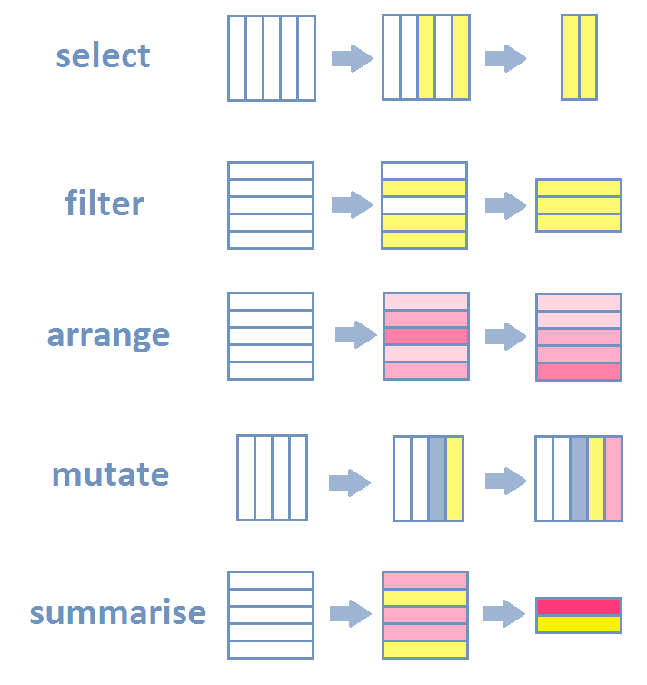
dplyr is a tool box for working with data in tibbles, offering a unified language for operations scattered through base R.

Key operations

This lecture

Example data

Van ’t Veer, Anna; Sleegers, Willem, 2019, “Psychology data from an exploration of the effect of anticipatory stress on disgust vs. non-disgust related moral judgments”. Journal of Open Psychology Data.

Data is not really tidy.
Typical data you might see in the wild.

Learning objectives

Learn the grammar to operate on rows and columns of a table
Selection and manipulation of
- observations,
- variables and
- values.
Grouping and summarizing
Joining and intersecting tibbles
Pivoting column headers and variables

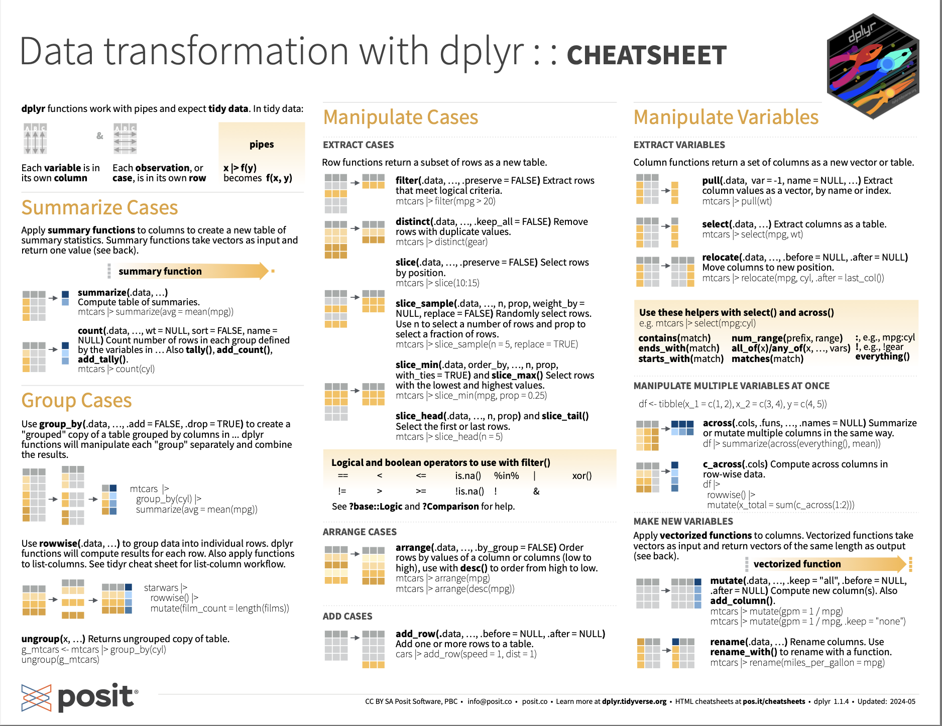
Key operations

`dplyr` Introduction: Cheat sheets

Using the `dplyr` package

Do not use these packages!

dplyr supersedes previous packages from Hadley Wickham.
- reshape
- reshape2
- plyr
All functionality can be found in dplyr or tidyr.

dplyr current version is 1.1.4

dplyr has seen many changes.
Watch out for deprecated examples on Stack overflow!
Code will break sooner or later (you might get lucky)
But handled with clear lifecycle stages now
Changes are generally introduced to simplify operations.

Loading dplyr

library(dplyr) # AND
library(tidyr)

# OR (recommended here) 

library(tidyverse)

Preparing the data

Description

Van ’t Veer, Anna; Sleegers, Willem. (2019) “Psychology data from an exploration of the effect of anticipatory stress on disgust vs. non-disgust related moral judgments”. Journal of Open Psychology Data.

Moral dilemmata (trolley problem, survival after plane crash, etc. moral)
Standard questionnaires
- Private Body Consciousness (PBC, range 0 - 4)
- Rational-Experiential Inventory (REI, range 1 - 5)
- Multidimensional Assessment of Interoceptive Awareness (MAIA, range 0 - 5 )
- State Trait Anxiety Inventory (STAI)

judge_url <- "https://biostat2.uni.lu/practicals/data/judgments.tsv"
judgments <- readr::read_tsv(judge_url)
# https://dataverse.nl/api/access/datafile/11863
#"https://biostat2.uni.lu/practicals/data/judgments.tsv")

Your turn!

Load the data into your RStudio session if you wish to follow along

02:00

judgments <- readr::read_tsv("https://biostat2.uni.lu/practicals/data/judgments.tsv", show_col_types = FALSE)
judgments

# A tibble: 188 × 158
   start_date end_date  finished condition subject
   <chr>      <chr>        <dbl> <chr>       <dbl>
 1 11/3/2014  11/3/2014        1 control         2
 2 11/3/2014  11/3/2014        1 stress          1
 3 11/3/2014  11/3/2014        1 stress          3
 4 11/3/2014  11/3/2014        1 stress          4
 5 11/3/2014  11/3/2014        1 control         7
 6 11/3/2014  11/3/2014        1 stress          6
 7 11/3/2014  11/3/2014        1 control         5
 8 11/3/2014  11/3/2014        1 control         9
 9 11/3/2014  11/3/2014        1 stress         16
10 11/3/2014  11/3/2014        1 stress         13
# ℹ 178 more rows
# ℹ 153 more variables: gender <chr>, age <dbl>,
#   mood_pre <dbl>, mood_post <dbl>,
#   STAI_pre_1_1 <dbl>, STAI_pre_1_2 <dbl>,
#   STAI_pre_1_3 <dbl>, STAI_pre_1_4 <dbl>,
#   STAI_pre_1_5 <dbl>, STAI_pre_1_6 <dbl>,
#   STAI_pre_1_7 <dbl>, STAI_pre_2_1 <dbl>, …

Inspecting tibbles

Inspect tibbles with `glimpse()`

Column-wise description

Shows some values and the type of each column.

The Environment tab in RStudio tab does it too.

Clicking object judgments triggers View().

Similar to the utils::str() function

glimpse(judgments)

Rows: 188
Columns: 158
$ start_date                 <chr> "11/3/2014", …
$ end_date                   <chr> "11/3/2014", …
$ finished                   <dbl> 1, 1, 1, 1, 1…
$ condition                  <chr> "control", "s…
$ subject                    <dbl> 2, 1, 3, 4, 7…
$ gender                     <chr> "female", "fe…
$ age                        <dbl> 24, 19, 19, 2…
$ mood_pre                   <dbl> 81, 59, 22, 5…
$ mood_post                  <dbl> NA, 42, 60, 6…
$ STAI_pre_1_1               <dbl> 2, 3, 4, 2, 1…
$ STAI_pre_1_2               <dbl> 1, 2, 3, 2, 1…
$ STAI_pre_1_3               <dbl> 2, 3, 3, 2, 1…
$ STAI_pre_1_4               <dbl> 2, 1, 3, 2, 1…
$ STAI_pre_1_5               <dbl> 2, 3, 4, 3, 2…
$ STAI_pre_1_6               <dbl> 2, 2, 2, 1, 1…
$ STAI_pre_1_7               <dbl> 2, 3, 3, 1, 1…
$ STAI_pre_2_1               <dbl> 2, 3, 4, 3, 3…
$ STAI_pre_2_2               <dbl> 1, 2, 2, 1, 1…
$ STAI_pre_2_3               <dbl> 1, 2, 3, 3, 3…
$ STAI_pre_2_4               <dbl> 1, 2, 4, 3, 3…
$ STAI_pre_2_5               <dbl> 1, 2, 4, 1, 1…
$ STAI_pre_2_6               <dbl> 1, 3, 4, 1, 1…
$ STAI_pre_2_7               <dbl> 1, 1, 2, 2, 1…
$ STAI_pre_3_1               <dbl> 2, 3, 4, 3, 1…
$ STAI_pre_3_2               <dbl> 2, 3, 3, 3, 2…
$ STAI_pre_3_3               <dbl> 2, 3, 2, 2, 2…
$ STAI_pre_3_4               <dbl> 1, 2, 3, 1, 1…
$ STAI_pre_3_5               <dbl> 2, 3, 4, 3, 3…
$ STAI_pre_3_6               <dbl> 2, 3, 4, 3, 3…
$ STAI_post_1_1              <dbl> NA, 3, 3, 2, …
$ STAI_post_1_2              <dbl> NA, 3, 3, 2, …
$ STAI_post_1_3              <dbl> NA, 3, 2, 1, …
$ STAI_post_1_4              <dbl> NA, 3, 2, 1, …
$ STAI_post_1_5              <dbl> NA, 2, 2, 2, …
$ STAI_post_1_6              <dbl> NA, 2, 1, 1, …
$ STAI_post_1_7              <dbl> NA, 3, 1, 1, …
$ STAI_post_2_1              <dbl> NA, 2, 3, 2, …
$ STAI_post_2_2              <dbl> NA, 2, 1, 1, …
$ STAI_post_2_3              <dbl> NA, 3, 3, 2, …
$ STAI_post_2_4              <dbl> NA, 3, 3, 2, …
$ STAI_post_2_5              <dbl> NA, 3, 1, 1, …
$ STAI_post_2_6              <dbl> NA, 3, 1, 1, …
$ STAI_post_2_7              <dbl> NA, 1, 1, 2, …
$ STAI_post_3_1              <dbl> NA, 2, 3, 2, …
$ STAI_post_3_2              <dbl> NA, 2, 3, 2, …
$ STAI_post_3_3              <dbl> NA, 3, 1, 1, …
$ STAI_post_3_4              <dbl> NA, 2, 1, 1, …
$ STAI_post_3_5              <dbl> NA, 3, 3, 3, …
$ STAI_post_3_6              <dbl> NA, 3, 3, 2, …
$ moral_dilemma_dog          <dbl> 9, 9, 8, 8, 3…
$ moral_dilemma_wallet       <dbl> 9, 9, 7, 4, 9…
$ moral_dilemma_plane        <dbl> 8, 9, 8, 8, 9…
$ moral_dilemma_resume       <dbl> 7, 8, 5, 6, 5…
$ moral_dilemma_kitten       <dbl> 9, 9, 8, 9, 5…
$ moral_dilemma_trolley      <dbl> 5, 3, 5, 2, 4…
$ moral_dilemma_control      <dbl> 9, 2, 9, 8, 8…
$ presentation_experience    <dbl> NA, 2, 1, 2, …
$ presentation_unpleasant    <dbl> NA, 63, 68, 3…
$ presentation_fun           <dbl> NA, 58, 26, 5…
$ presentation_challenge     <dbl> NA, 58, 65, 8…
$ PBC_1                      <dbl> 3, NA, NA, NA…
$ PBC_2                      <dbl> 3, NA, NA, NA…
$ PBC_3                      <dbl> 5, NA, NA, NA…
$ PBC_4                      <dbl> 5, NA, NA, NA…
$ PBC_5                      <dbl> 5, NA, NA, NA…
$ REI_1                      <dbl> 5, NA, NA, NA…
$ REI_2                      <dbl> 4, NA, NA, NA…
$ REI_3                      <dbl> 5, NA, NA, NA…
$ REI_4                      <dbl> 4, NA, NA, NA…
$ REI_5                      <dbl> 4, NA, NA, NA…
$ REI_6                      <dbl> 5, NA, NA, NA…
$ REI_7                      <dbl> 3, NA, NA, NA…
$ REI_8                      <dbl> 4, NA, NA, NA…
$ REI_9                      <dbl> 3, NA, NA, NA…
$ REI_10                     <dbl> 4, NA, NA, NA…
$ REI_11                     <dbl> 5, NA, NA, NA…
$ REI_12                     <dbl> 5, NA, NA, NA…
$ REI_13                     <dbl> 3, NA, NA, NA…
$ REI_14                     <dbl> 4, NA, NA, NA…
$ REI_15                     <dbl> 4, NA, NA, NA…
$ REI_16                     <dbl> 4, NA, NA, NA…
$ REI_17                     <dbl> 3, NA, NA, NA…
$ REI_18                     <dbl> 5, NA, NA, NA…
$ REI_19                     <dbl> 1, NA, NA, NA…
$ REI_20                     <dbl> 3, NA, NA, NA…
$ REI_21                     <dbl> 5, NA, NA, NA…
$ REI_22                     <dbl> 3, NA, NA, NA…
$ REI_23                     <dbl> 4, NA, NA, NA…
$ REI_24                     <dbl> 2, NA, NA, NA…
$ REI_25                     <dbl> 3, NA, NA, NA…
$ REI_26                     <dbl> 5, NA, NA, NA…
$ REI_27                     <dbl> 5, NA, NA, NA…
$ REI_28                     <dbl> 3, NA, NA, NA…
$ REI_29                     <dbl> 3, NA, NA, NA…
$ REI_30                     <dbl> 4, NA, NA, NA…
$ REI_31                     <dbl> 3, NA, NA, NA…
$ REI_32                     <dbl> 3, NA, NA, NA…
$ REI_33                     <dbl> 4, NA, NA, NA…
$ REI_34                     <dbl> 3, NA, NA, NA…
$ REI_35                     <dbl> 4, NA, NA, NA…
$ REI_36                     <dbl> 3, NA, NA, NA…
$ REI_37                     <dbl> 4, NA, NA, NA…
$ REI_38                     <dbl> 4, NA, NA, NA…
$ REI_39                     <dbl> 4, NA, NA, NA…
$ REI_40                     <dbl> 4, NA, NA, NA…
$ MAIA_1_1                   <dbl> 2, NA, NA, NA…
$ MAIA_1_2                   <dbl> 4, NA, NA, NA…
$ MAIA_1_3                   <dbl> 4, NA, NA, NA…
$ MAIA_1_4                   <dbl> 4, NA, NA, NA…
$ MAIA_1_5                   <dbl> 2, NA, NA, NA…
$ MAIA_1_6                   <dbl> 2, NA, NA, NA…
$ MAIA_1_7                   <dbl> 2, NA, NA, NA…
$ MAIA_1_8                   <dbl> 3, NA, NA, NA…
$ MAIA_1_9                   <dbl> 4, NA, NA, NA…
$ MAIA_1_10                  <dbl> 4, NA, NA, NA…
$ MAIA_1_11                  <dbl> 4, NA, NA, NA…
$ MAIA_1_12                  <dbl> 3, NA, NA, NA…
$ MAIA_1_13                  <dbl> 4, NA, NA, NA…
$ MAIA_1_14                  <dbl> 4, NA, NA, NA…
$ MAIA_1_15                  <dbl> 4, NA, NA, NA…
$ MAIA_1_16                  <dbl> 4, NA, NA, NA…
$ MAIA_2_1                   <dbl> 4, NA, NA, NA…
$ MAIA_2_2                   <dbl> 4, NA, NA, NA…
$ MAIA_2_3                   <dbl> 4, NA, NA, NA…
$ MAIA_2_4                   <dbl> 4, NA, NA, NA…
$ MAIA_2_5                   <dbl> 4, NA, NA, NA…
$ MAIA_2_6                   <dbl> 4, NA, NA, NA…
$ MAIA_2_7                   <dbl> 4, NA, NA, NA…
$ MAIA_2_8                   <dbl> 4, NA, NA, NA…
$ MAIA_2_9                   <dbl> 4, NA, NA, NA…
$ MAIA_2_10                  <dbl> 4, NA, NA, NA…
$ MAIA_2_11                  <dbl> 4, NA, NA, NA…
$ MAIA_2_12                  <dbl> 3, NA, NA, NA…
$ MAIA_2_13                  <dbl> 3, NA, NA, NA…
$ MAIA_2_14                  <dbl> 4, NA, NA, NA…
$ MAIA_2_15                  <dbl> 4, NA, NA, NA…
$ MAIA_2_16                  <dbl> 4, NA, NA, NA…
$ STAI_pre                   <dbl> 32, 49, 65, 4…
$ STAI_post                  <dbl> NA, 51, 41, 3…
$ MAIA_noticing              <dbl> 14, NA, NA, N…
$ MAIA_not_distracting       <dbl> 6, NA, NA, NA…
$ MAIA_not_worrying          <dbl> 11, NA, NA, N…
$ MAIA_attention_regulation  <dbl> 27, NA, NA, N…
$ MAIA_emotional_awareness   <dbl> 20, NA, NA, N…
$ MAIA_self_regulation       <dbl> 16, NA, NA, N…
$ MAIA_body_listening        <dbl> 10, NA, NA, N…
$ MAIA_trusting              <dbl> 12, NA, NA, N…
$ PBC                        <dbl> 21, NA, NA, N…
$ REI_rational_ability       <dbl> 38, NA, NA, N…
$ REI_rational_engagement    <dbl> 38, NA, NA, N…
$ REI_experiental_ability    <dbl> 36, NA, NA, N…
$ REI_experiental_engagement <dbl> 39, NA, NA, N…
$ moral_judgment             <dbl> 8.000000, 7.0…
$ moral_judgment_disgust     <dbl> 8.666667, 9.0…
$ moral_judgment_non_disgust <dbl> 7.000000, 6.6…
$ presentation_evaluation    <dbl> NA, 3, 3, 4, …
$ logbook                    <chr> NA, NA, NA, N…
$ exclude                    <dbl> 0, 0, 0, 0, 0…

Selecting columns

select(tibble, column1, ...)

select(judgments, gender, age, condition)

# A tibble: 188 × 3
   gender   age condition
   <chr>  <dbl> <chr>    
 1 female    24 control  
 2 female    19 stress   
 3 female    19 stress   
 4 female    22 stress   
 5 female    22 control  
 6 female    22 stress   
 7 female    18 control  
 8 male      20 control  
 9 female    21 stress   
10 female    19 stress   
# ℹ 178 more rows

Non-standard evaluation

Note the absence of quotes around column names!

Warning

The biomaRt package of Bioconductor (amongst others) provides a select() function. If loaded, we need to address the dplyr-package using ::!

dplyr::select(judgments, age, gender)

# A tibble: 188 × 2
     age gender
   <dbl> <chr> 
 1    24 female
 2    19 female
 3    19 female
 4    22 female
 5    22 female
 6    22 female
 7    18 female
 8    20 male  
 9    21 female
10    19 female
# ℹ 178 more rows

Reminder `tidyselect`

Helper function

To select columns with names that:

contains() - a string
starts_with() - a string
ends_with() - a string
any_of() - any names in a character vectorc("col_name")
all_of() - all names in a character vector c("col_name")
matches() - using regular expressions
everything() - all remaining columns
last_col() - last column

Avoid selecting columns by index!

To ensure reproducibility select columns by name

select(judgments, starts_with("moral"))

# A tibble: 188 × 10
   moral_dilemma_dog moral_dilemma_wallet
               <dbl>                <dbl>
 1                 9                    9
 2                 9                    9
 3                 8                    7
 4                 8                    4
 5                 3                    9
 6                 9                    9
 7                 9                    5
 8                 9                    4
 9                 6                    9
10                 6                    8
# ℹ 178 more rows
# ℹ 8 more variables: moral_dilemma_plane <dbl>,
#   moral_dilemma_resume <dbl>,
#   moral_dilemma_kitten <dbl>,
#   moral_dilemma_trolley <dbl>,
#   moral_dilemma_control <dbl>,
#   moral_judgment <dbl>, …

Combining helpers

Remark

Helpers are found in several functions, e.g. across().

select(judgments, ends_with("date"), contains("dilemma"))

# A tibble: 188 × 9
   start_date end_date  moral_dilemma_dog
   <chr>      <chr>                 <dbl>
 1 11/3/2014  11/3/2014                 9
 2 11/3/2014  11/3/2014                 9
 3 11/3/2014  11/3/2014                 8
 4 11/3/2014  11/3/2014                 8
 5 11/3/2014  11/3/2014                 3
 6 11/3/2014  11/3/2014                 9
 7 11/3/2014  11/3/2014                 9
 8 11/3/2014  11/3/2014                 9
 9 11/3/2014  11/3/2014                 6
10 11/3/2014  11/3/2014                 6
# ℹ 178 more rows
# ℹ 6 more variables: moral_dilemma_wallet <dbl>,
#   moral_dilemma_plane <dbl>,
#   moral_dilemma_resume <dbl>,
#   moral_dilemma_kitten <dbl>,
#   moral_dilemma_trolley <dbl>,
#   moral_dilemma_control <dbl>

Selecting with quoted names

vars <- c("moral_dilemma_control", 
          "moral_dilemma_trump")
select(judgments, subject, any_of(vars))

# A tibble: 188 × 2
   subject moral_dilemma_control
     <dbl>                 <dbl>
 1       2                     9
 2       1                     2
 3       3                     9
 4       4                     8
 5       7                     8
 6       6                     6
 7       5                     8
 8       9                     7
 9      16                     8
10      13                     6
# ℹ 178 more rows

select(judgments, subject, all_of(vars))

Error in `all_of()`:
! Can't subset columns that don't exist.
✖ Column `moral_dilemma_trump` doesn't exist.

Helpers are evaluated from left to right

Order of selection matters!

select(judgments, starts_with("STAI"), -contains("pre"))

# A tibble: 188 × 21
   STAI_post_1_1 STAI_post_1_2 STAI_post_1_3
           <dbl>         <dbl>         <dbl>
 1            NA            NA            NA
 2             3             3             3
 3             3             3             2
 4             2             2             1
 5            NA            NA            NA
 6             2             2             1
 7            NA            NA            NA
 8            NA            NA            NA
 9             2             2             1
10             2             2             1
# ℹ 178 more rows
# ℹ 18 more variables: STAI_post_1_4 <dbl>,
#   STAI_post_1_5 <dbl>, STAI_post_1_6 <dbl>,
#   STAI_post_1_7 <dbl>, STAI_post_2_1 <dbl>,
#   STAI_post_2_2 <dbl>, STAI_post_2_3 <dbl>,
#   STAI_post_2_4 <dbl>, STAI_post_2_5 <dbl>,
#   STAI_post_2_6 <dbl>, STAI_post_2_7 <dbl>, …

select(judgments, -contains("pre"), starts_with("STAI"))

# A tibble: 188 × 152
   start_date end_date  finished condition subject
   <chr>      <chr>        <dbl> <chr>       <dbl>
 1 11/3/2014  11/3/2014        1 control         2
 2 11/3/2014  11/3/2014        1 stress          1
 3 11/3/2014  11/3/2014        1 stress          3
 4 11/3/2014  11/3/2014        1 stress          4
 5 11/3/2014  11/3/2014        1 control         7
 6 11/3/2014  11/3/2014        1 stress          6
 7 11/3/2014  11/3/2014        1 control         5
 8 11/3/2014  11/3/2014        1 control         9
 9 11/3/2014  11/3/2014        1 stress         16
10 11/3/2014  11/3/2014        1 stress         13
# ℹ 178 more rows
# ℹ 147 more variables: gender <chr>, age <dbl>,
#   mood_post <dbl>, STAI_post_1_1 <dbl>,
#   STAI_post_1_2 <dbl>, STAI_post_1_3 <dbl>,
#   STAI_post_1_4 <dbl>, STAI_post_1_5 <dbl>,
#   STAI_post_1_6 <dbl>, STAI_post_1_7 <dbl>,
#   STAI_post_2_1 <dbl>, STAI_post_2_2 <dbl>, …

Selecting columns

Negative selection

Drop columns by negating their names -

Works with the tidyselect helper functions.

select(judgments, 
       -gender, 
       -starts_with(c("STAI", "REI")),
       -ends_with("id"))

# A tibble: 188 × 71
   start_date end_date  finished condition subject
   <chr>      <chr>        <dbl> <chr>       <dbl>
 1 11/3/2014  11/3/2014        1 control         2
 2 11/3/2014  11/3/2014        1 stress          1
 3 11/3/2014  11/3/2014        1 stress          3
 4 11/3/2014  11/3/2014        1 stress          4
 5 11/3/2014  11/3/2014        1 control         7
 6 11/3/2014  11/3/2014        1 stress          6
 7 11/3/2014  11/3/2014        1 control         5
 8 11/3/2014  11/3/2014        1 control         9
 9 11/3/2014  11/3/2014        1 stress         16
10 11/3/2014  11/3/2014        1 stress         13
# ℹ 178 more rows
# ℹ 66 more variables: age <dbl>, mood_pre <dbl>,
#   mood_post <dbl>, moral_dilemma_dog <dbl>,
#   moral_dilemma_wallet <dbl>,
#   moral_dilemma_plane <dbl>,
#   moral_dilemma_resume <dbl>,
#   moral_dilemma_kitten <dbl>, …

`relocate()`

.before and .after for fine placement. Works also with mutate()

judgments |> relocate(contains("STA"))

# A tibble: 188 × 158
   start_date STAI_pre_1_1 STAI_pre_1_2
   <chr>             <dbl>        <dbl>
 1 11/3/2014             2            1
 2 11/3/2014             3            2
 3 11/3/2014             4            3
 4 11/3/2014             2            2
 5 11/3/2014             1            1
 6 11/3/2014             2            2
 7 11/3/2014             2            2
 8 11/3/2014             1            1
 9 11/3/2014             2            2
10 11/3/2014             4            2
# ℹ 178 more rows
# ℹ 155 more variables: STAI_pre_1_3 <dbl>,
#   STAI_pre_1_4 <dbl>, STAI_pre_1_5 <dbl>,
#   STAI_pre_1_6 <dbl>, STAI_pre_1_7 <dbl>,
#   STAI_pre_2_1 <dbl>, STAI_pre_2_2 <dbl>,
#   STAI_pre_2_3 <dbl>, STAI_pre_2_4 <dbl>,
#   STAI_pre_2_5 <dbl>, STAI_pre_2_6 <dbl>, …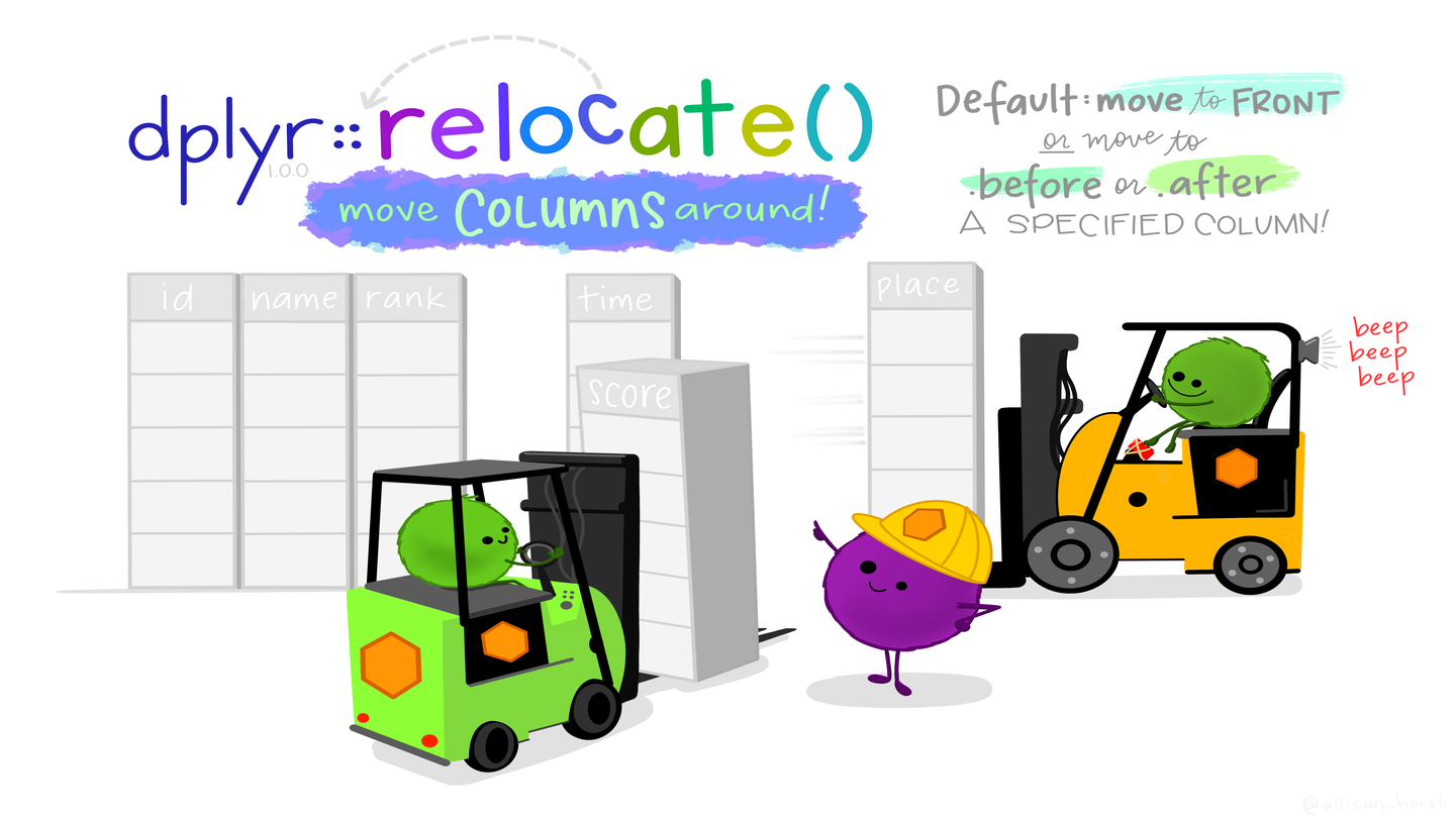

Filtering for rows: `filter()`

Let’s take a look at all the data that was excluded. The column exclude is coded as \(0=include\) and \(1=exclude\).

filter(judgments, exclude == 1)

# A tibble: 3 × 158
  start_date end_date  finished condition subject
  <chr>      <chr>        <dbl> <chr>       <dbl>
1 11/3/2014  11/3/2014        1 stress         28
2 11/3/2014  11/3/2014        1 stress         32
3 11/7/2014  11/7/2014        1 stress        181
# ℹ 153 more variables: gender <chr>, age <dbl>,
#   mood_pre <dbl>, mood_post <dbl>,
#   STAI_pre_1_1 <dbl>, STAI_pre_1_2 <dbl>,
#   STAI_pre_1_3 <dbl>, STAI_pre_1_4 <dbl>,
#   STAI_pre_1_5 <dbl>, STAI_pre_1_6 <dbl>,
#   STAI_pre_1_7 <dbl>, STAI_pre_2_1 <dbl>,
#   STAI_pre_2_2 <dbl>, STAI_pre_2_3 <dbl>, …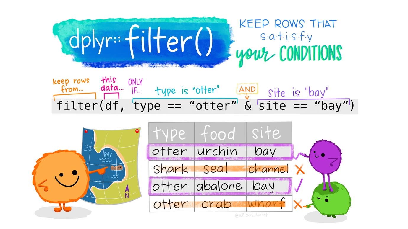

Filtering rows

Multiple conditions: AND

comma separated conditions are equivalent to & (AND).
Filter for females older than 20.

filter(judgments,
  age > 20,
  gender == "female")

# A tibble: 34 × 158
   start_date end_date  finished condition subject
   <chr>      <chr>        <dbl> <chr>       <dbl>
 1 11/3/2014  11/3/2014        1 control         2
 2 11/3/2014  11/3/2014        1 stress          4
 3 11/3/2014  11/3/2014        1 control         7
 4 11/3/2014  11/3/2014        1 stress          6
 5 11/3/2014  11/3/2014        1 stress         16
 6 11/3/2014  11/3/2014        1 control        10
 7 11/3/2014  11/3/2014        1 control        23
 8 11/3/2014  11/3/2014        1 control        29
 9 11/3/2014  11/3/2014        1 stress         36
10 11/3/2014  11/3/2014        1 control        31
# ℹ 24 more rows
# ℹ 153 more variables: gender <chr>, age <dbl>,
#   mood_pre <dbl>, mood_post <dbl>,
#   STAI_pre_1_1 <dbl>, STAI_pre_1_2 <dbl>,
#   STAI_pre_1_3 <dbl>, STAI_pre_1_4 <dbl>,
#   STAI_pre_1_5 <dbl>, STAI_pre_1_6 <dbl>,
#   STAI_pre_1_7 <dbl>, STAI_pre_2_1 <dbl>, …

Multiple conditions: OR

vertical bar (|) separated conditions are combined with OR.
Filter females or age > 20 (so males too)

filter(judgments,
  age > 20 |
  gender == "female")

# A tibble: 164 × 158
   start_date end_date  finished condition subject
   <chr>      <chr>        <dbl> <chr>       <dbl>
 1 11/3/2014  11/3/2014        1 control         2
 2 11/3/2014  11/3/2014        1 stress          1
 3 11/3/2014  11/3/2014        1 stress          3
 4 11/3/2014  11/3/2014        1 stress          4
 5 11/3/2014  11/3/2014        1 control         7
 6 11/3/2014  11/3/2014        1 stress          6
 7 11/3/2014  11/3/2014        1 control         5
 8 11/3/2014  11/3/2014        1 stress         16
 9 11/3/2014  11/3/2014        1 stress         13
10 11/3/2014  11/3/2014        1 stress         18
# ℹ 154 more rows
# ℹ 153 more variables: gender <chr>, age <dbl>,
#   mood_pre <dbl>, mood_post <dbl>,
#   STAI_pre_1_1 <dbl>, STAI_pre_1_2 <dbl>,
#   STAI_pre_1_3 <dbl>, STAI_pre_1_4 <dbl>,
#   STAI_pre_1_5 <dbl>, STAI_pre_1_6 <dbl>,
#   STAI_pre_1_7 <dbl>, STAI_pre_2_1 <dbl>, …

Filtering out rows

Row vs column selection

filter() acts on rows
select() acts on columns

Remove excluded participants
Combine with relocate() to place mood columns first

filter(judgments, exclude == 0) |> 
  relocate(contains("mood"))

# A tibble: 185 × 158
   mood_pre mood_post start_date end_date finished
      <dbl>     <dbl> <chr>      <chr>       <dbl>
 1       81        NA 11/3/2014  11/3/20…        1
 2       59        42 11/3/2014  11/3/20…        1
 3       22        60 11/3/2014  11/3/20…        1
 4       53        68 11/3/2014  11/3/20…        1
 5       48        NA 11/3/2014  11/3/20…        1
 6       73        73 11/3/2014  11/3/20…        1
 7       NA        NA 11/3/2014  11/3/20…        1
 8      100        NA 11/3/2014  11/3/20…        1
 9       67        74 11/3/2014  11/3/20…        1
10       30        68 11/3/2014  11/3/20…        1
# ℹ 175 more rows
# ℹ 153 more variables: condition <chr>,
#   subject <dbl>, gender <chr>, age <dbl>,
#   STAI_pre_1_1 <dbl>, STAI_pre_1_2 <dbl>,
#   STAI_pre_1_3 <dbl>, STAI_pre_1_4 <dbl>,
#   STAI_pre_1_5 <dbl>, STAI_pre_1_6 <dbl>,
#   STAI_pre_1_7 <dbl>, STAI_pre_2_1 <dbl>, …

Filter rows, helper `between()`

judgments |>
  filter(between(mood_pre, 40, 60)) |> 
  select(age, gender, condition, mood_pre)

# A tibble: 64 × 4
     age gender condition mood_pre
   <dbl> <chr>  <chr>        <dbl>
 1    19 female stress          59
 2    22 female stress          53
 3    22 female control         48
 4    19 female stress          55
 5    18 female stress          53
 6    19 female control         59
 7    19 female stress          60
 8    22 male   stress          53
 9    18 male   control         50
10    19 female stress          58
# ℹ 54 more rows

Set operations with `filter()`

judgments |>
  filter(is.element(start_date, c("11/3/2014", "11/5/2014"))) |>
  select(start_date:age)

# A tibble: 79 × 7
   start_date end_date  finished condition subject
   <chr>      <chr>        <dbl> <chr>       <dbl>
 1 11/3/2014  11/3/2014        1 control         2
 2 11/3/2014  11/3/2014        1 stress          1
 3 11/3/2014  11/3/2014        1 stress          3
 4 11/3/2014  11/3/2014        1 stress          4
 5 11/3/2014  11/3/2014        1 control         7
 6 11/3/2014  11/3/2014        1 stress          6
 7 11/3/2014  11/3/2014        1 control         5
 8 11/3/2014  11/3/2014        1 control         9
 9 11/3/2014  11/3/2014        1 stress         16
10 11/3/2014  11/3/2014        1 stress         13
# ℹ 69 more rows
# ℹ 2 more variables: gender <chr>, age <dbl>

Not efficient for large data sets

For larger operations use filtering joins such as semi_join().

judgments |>
  filter(start_date %in% c("11/3/2014", "11/5/2014")) |>
  select(start_date:age)

# A tibble: 79 × 7
   start_date end_date  finished condition subject
   <chr>      <chr>        <dbl> <chr>       <dbl>
 1 11/3/2014  11/3/2014        1 control         2
 2 11/3/2014  11/3/2014        1 stress          1
 3 11/3/2014  11/3/2014        1 stress          3
 4 11/3/2014  11/3/2014        1 stress          4
 5 11/3/2014  11/3/2014        1 control         7
 6 11/3/2014  11/3/2014        1 stress          6
 7 11/3/2014  11/3/2014        1 control         5
 8 11/3/2014  11/3/2014        1 control         9
 9 11/3/2014  11/3/2014        1 stress         16
10 11/3/2014  11/3/2014        1 stress         13
# ℹ 69 more rows
# ℹ 2 more variables: gender <chr>, age <dbl>

Filter out rows that are unique: `distinct()`

Do we have different start / end dates?

select(judgments, start_date, end_date)

# A tibble: 188 × 2
   start_date end_date 
   <chr>      <chr>    
 1 11/3/2014  11/3/2014
 2 11/3/2014  11/3/2014
 3 11/3/2014  11/3/2014
 4 11/3/2014  11/3/2014
 5 11/3/2014  11/3/2014
 6 11/3/2014  11/3/2014
 7 11/3/2014  11/3/2014
 8 11/3/2014  11/3/2014
 9 11/3/2014  11/3/2014
10 11/3/2014  11/3/2014
# ℹ 178 more rows

Too many identical rows

Use `distinct()` to remove duplicated rows:

judgments |>
  filter(exclude == 0) |> 
  select(start_date, end_date) |> 
  distinct()

# A tibble: 5 × 2
  start_date end_date 
  <chr>      <chr>    
1 11/3/2014  11/3/2014
2 11/4/2014  11/4/2014
3 11/5/2014  11/5/2014
4 11/6/2014  11/6/2014
5 11/7/2014  11/7/2014

Also possible (except columns order):

judgments |>
  filter(exclude == 0) |> 
  distinct(start_date, end_date)

Sort columns: `arrange()`

A nested sorting example

Sort by age
Within each group of age, sort by mood_post

judgments |> 
  arrange(age, mood_post) |> 
  select(subject, age, mood_post)

# A tibble: 188 × 3
   subject   age mood_post
     <dbl> <dbl>     <dbl>
 1      81    17        11
 2      15    17        38
 3      58    17        60
 4     174    17        76
 5     147    17        82
 6      33    17        NA
 7      55    17        NA
 8     143    17        NA
 9     159    18         0
10     127    18        20
# ℹ 178 more rows

Reverse sort columns

Use arrange() with the helper function desc()
For example, oldest participant first

judgments |> 
  arrange(desc(age), mood_post) |> 
  select(subject, age, mood_post)

# A tibble: 188 × 3
   subject   age mood_post
     <dbl> <dbl>     <dbl>
 1     107    31        99
 2      61    27        64
 3      41    26        NA
 4     183    25        94
 5     115    24        79
 6      93    24       100
 7       2    24        NA
 8     137    24        NA
 9      86    23        62
10      49    23        75
# ℹ 178 more rows

Verbs to inspect data

Summary

glimpse() to get an overview of each column’s content
select() to pick and/or omit columns
- helper functions
relocate() re-arrange columns order
filter() to subset
- AND/OR conditions (,, |)
arrange() to sort
- combine with desc() to reverse the sorting

Your turn!

Exercises

Use glimpse() to identify columns and column types in judgments.
Select all columns that refer to the STAI questionnaire.
Retrieve all subjects younger than 20 which are in the stress group. The column for the group is condition.
Arrange all observations by STAI_pre so that the subject with the lowest score is on top. What is the subject in question?

05:00

Solution

glimpse(judgments)

Rows: 188
Columns: 158
$ start_date                 <chr> "11/3/2014", …
$ end_date                   <chr> "11/3/2014", …
$ finished                   <dbl> 1, 1, 1, 1, 1…
$ condition                  <chr> "control", "s…
$ subject                    <dbl> 2, 1, 3, 4, 7…
$ gender                     <chr> "female", "fe…
$ age                        <dbl> 24, 19, 19, 2…
$ mood_pre                   <dbl> 81, 59, 22, 5…
$ mood_post                  <dbl> NA, 42, 60, 6…
$ STAI_pre_1_1               <dbl> 2, 3, 4, 2, 1…
$ STAI_pre_1_2               <dbl> 1, 2, 3, 2, 1…
$ STAI_pre_1_3               <dbl> 2, 3, 3, 2, 1…
$ STAI_pre_1_4               <dbl> 2, 1, 3, 2, 1…
$ STAI_pre_1_5               <dbl> 2, 3, 4, 3, 2…
$ STAI_pre_1_6               <dbl> 2, 2, 2, 1, 1…
$ STAI_pre_1_7               <dbl> 2, 3, 3, 1, 1…
$ STAI_pre_2_1               <dbl> 2, 3, 4, 3, 3…
$ STAI_pre_2_2               <dbl> 1, 2, 2, 1, 1…
$ STAI_pre_2_3               <dbl> 1, 2, 3, 3, 3…
$ STAI_pre_2_4               <dbl> 1, 2, 4, 3, 3…
$ STAI_pre_2_5               <dbl> 1, 2, 4, 1, 1…
$ STAI_pre_2_6               <dbl> 1, 3, 4, 1, 1…
$ STAI_pre_2_7               <dbl> 1, 1, 2, 2, 1…
$ STAI_pre_3_1               <dbl> 2, 3, 4, 3, 1…
$ STAI_pre_3_2               <dbl> 2, 3, 3, 3, 2…
$ STAI_pre_3_3               <dbl> 2, 3, 2, 2, 2…
$ STAI_pre_3_4               <dbl> 1, 2, 3, 1, 1…
$ STAI_pre_3_5               <dbl> 2, 3, 4, 3, 3…
$ STAI_pre_3_6               <dbl> 2, 3, 4, 3, 3…
$ STAI_post_1_1              <dbl> NA, 3, 3, 2, …
$ STAI_post_1_2              <dbl> NA, 3, 3, 2, …
$ STAI_post_1_3              <dbl> NA, 3, 2, 1, …
$ STAI_post_1_4              <dbl> NA, 3, 2, 1, …
$ STAI_post_1_5              <dbl> NA, 2, 2, 2, …
$ STAI_post_1_6              <dbl> NA, 2, 1, 1, …
$ STAI_post_1_7              <dbl> NA, 3, 1, 1, …
$ STAI_post_2_1              <dbl> NA, 2, 3, 2, …
$ STAI_post_2_2              <dbl> NA, 2, 1, 1, …
$ STAI_post_2_3              <dbl> NA, 3, 3, 2, …
$ STAI_post_2_4              <dbl> NA, 3, 3, 2, …
$ STAI_post_2_5              <dbl> NA, 3, 1, 1, …
$ STAI_post_2_6              <dbl> NA, 3, 1, 1, …
$ STAI_post_2_7              <dbl> NA, 1, 1, 2, …
$ STAI_post_3_1              <dbl> NA, 2, 3, 2, …
$ STAI_post_3_2              <dbl> NA, 2, 3, 2, …
$ STAI_post_3_3              <dbl> NA, 3, 1, 1, …
$ STAI_post_3_4              <dbl> NA, 2, 1, 1, …
$ STAI_post_3_5              <dbl> NA, 3, 3, 3, …
$ STAI_post_3_6              <dbl> NA, 3, 3, 2, …
$ moral_dilemma_dog          <dbl> 9, 9, 8, 8, 3…
$ moral_dilemma_wallet       <dbl> 9, 9, 7, 4, 9…
$ moral_dilemma_plane        <dbl> 8, 9, 8, 8, 9…
$ moral_dilemma_resume       <dbl> 7, 8, 5, 6, 5…
$ moral_dilemma_kitten       <dbl> 9, 9, 8, 9, 5…
$ moral_dilemma_trolley      <dbl> 5, 3, 5, 2, 4…
$ moral_dilemma_control      <dbl> 9, 2, 9, 8, 8…
$ presentation_experience    <dbl> NA, 2, 1, 2, …
$ presentation_unpleasant    <dbl> NA, 63, 68, 3…
$ presentation_fun           <dbl> NA, 58, 26, 5…
$ presentation_challenge     <dbl> NA, 58, 65, 8…
$ PBC_1                      <dbl> 3, NA, NA, NA…
$ PBC_2                      <dbl> 3, NA, NA, NA…
$ PBC_3                      <dbl> 5, NA, NA, NA…
$ PBC_4                      <dbl> 5, NA, NA, NA…
$ PBC_5                      <dbl> 5, NA, NA, NA…
$ REI_1                      <dbl> 5, NA, NA, NA…
$ REI_2                      <dbl> 4, NA, NA, NA…
$ REI_3                      <dbl> 5, NA, NA, NA…
$ REI_4                      <dbl> 4, NA, NA, NA…
$ REI_5                      <dbl> 4, NA, NA, NA…
$ REI_6                      <dbl> 5, NA, NA, NA…
$ REI_7                      <dbl> 3, NA, NA, NA…
$ REI_8                      <dbl> 4, NA, NA, NA…
$ REI_9                      <dbl> 3, NA, NA, NA…
$ REI_10                     <dbl> 4, NA, NA, NA…
$ REI_11                     <dbl> 5, NA, NA, NA…
$ REI_12                     <dbl> 5, NA, NA, NA…
$ REI_13                     <dbl> 3, NA, NA, NA…
$ REI_14                     <dbl> 4, NA, NA, NA…
$ REI_15                     <dbl> 4, NA, NA, NA…
$ REI_16                     <dbl> 4, NA, NA, NA…
$ REI_17                     <dbl> 3, NA, NA, NA…
$ REI_18                     <dbl> 5, NA, NA, NA…
$ REI_19                     <dbl> 1, NA, NA, NA…
$ REI_20                     <dbl> 3, NA, NA, NA…
$ REI_21                     <dbl> 5, NA, NA, NA…
$ REI_22                     <dbl> 3, NA, NA, NA…
$ REI_23                     <dbl> 4, NA, NA, NA…
$ REI_24                     <dbl> 2, NA, NA, NA…
$ REI_25                     <dbl> 3, NA, NA, NA…
$ REI_26                     <dbl> 5, NA, NA, NA…
$ REI_27                     <dbl> 5, NA, NA, NA…
$ REI_28                     <dbl> 3, NA, NA, NA…
$ REI_29                     <dbl> 3, NA, NA, NA…
$ REI_30                     <dbl> 4, NA, NA, NA…
$ REI_31                     <dbl> 3, NA, NA, NA…
$ REI_32                     <dbl> 3, NA, NA, NA…
$ REI_33                     <dbl> 4, NA, NA, NA…
$ REI_34                     <dbl> 3, NA, NA, NA…
$ REI_35                     <dbl> 4, NA, NA, NA…
$ REI_36                     <dbl> 3, NA, NA, NA…
$ REI_37                     <dbl> 4, NA, NA, NA…
$ REI_38                     <dbl> 4, NA, NA, NA…
$ REI_39                     <dbl> 4, NA, NA, NA…
$ REI_40                     <dbl> 4, NA, NA, NA…
$ MAIA_1_1                   <dbl> 2, NA, NA, NA…
$ MAIA_1_2                   <dbl> 4, NA, NA, NA…
$ MAIA_1_3                   <dbl> 4, NA, NA, NA…
$ MAIA_1_4                   <dbl> 4, NA, NA, NA…
$ MAIA_1_5                   <dbl> 2, NA, NA, NA…
$ MAIA_1_6                   <dbl> 2, NA, NA, NA…
$ MAIA_1_7                   <dbl> 2, NA, NA, NA…
$ MAIA_1_8                   <dbl> 3, NA, NA, NA…
$ MAIA_1_9                   <dbl> 4, NA, NA, NA…
$ MAIA_1_10                  <dbl> 4, NA, NA, NA…
$ MAIA_1_11                  <dbl> 4, NA, NA, NA…
$ MAIA_1_12                  <dbl> 3, NA, NA, NA…
$ MAIA_1_13                  <dbl> 4, NA, NA, NA…
$ MAIA_1_14                  <dbl> 4, NA, NA, NA…
$ MAIA_1_15                  <dbl> 4, NA, NA, NA…
$ MAIA_1_16                  <dbl> 4, NA, NA, NA…
$ MAIA_2_1                   <dbl> 4, NA, NA, NA…
$ MAIA_2_2                   <dbl> 4, NA, NA, NA…
$ MAIA_2_3                   <dbl> 4, NA, NA, NA…
$ MAIA_2_4                   <dbl> 4, NA, NA, NA…
$ MAIA_2_5                   <dbl> 4, NA, NA, NA…
$ MAIA_2_6                   <dbl> 4, NA, NA, NA…
$ MAIA_2_7                   <dbl> 4, NA, NA, NA…
$ MAIA_2_8                   <dbl> 4, NA, NA, NA…
$ MAIA_2_9                   <dbl> 4, NA, NA, NA…
$ MAIA_2_10                  <dbl> 4, NA, NA, NA…
$ MAIA_2_11                  <dbl> 4, NA, NA, NA…
$ MAIA_2_12                  <dbl> 3, NA, NA, NA…
$ MAIA_2_13                  <dbl> 3, NA, NA, NA…
$ MAIA_2_14                  <dbl> 4, NA, NA, NA…
$ MAIA_2_15                  <dbl> 4, NA, NA, NA…
$ MAIA_2_16                  <dbl> 4, NA, NA, NA…
$ STAI_pre                   <dbl> 32, 49, 65, 4…
$ STAI_post                  <dbl> NA, 51, 41, 3…
$ MAIA_noticing              <dbl> 14, NA, NA, N…
$ MAIA_not_distracting       <dbl> 6, NA, NA, NA…
$ MAIA_not_worrying          <dbl> 11, NA, NA, N…
$ MAIA_attention_regulation  <dbl> 27, NA, NA, N…
$ MAIA_emotional_awareness   <dbl> 20, NA, NA, N…
$ MAIA_self_regulation       <dbl> 16, NA, NA, N…
$ MAIA_body_listening        <dbl> 10, NA, NA, N…
$ MAIA_trusting              <dbl> 12, NA, NA, N…
$ PBC                        <dbl> 21, NA, NA, N…
$ REI_rational_ability       <dbl> 38, NA, NA, N…
$ REI_rational_engagement    <dbl> 38, NA, NA, N…
$ REI_experiental_ability    <dbl> 36, NA, NA, N…
$ REI_experiental_engagement <dbl> 39, NA, NA, N…
$ moral_judgment             <dbl> 8.000000, 7.0…
$ moral_judgment_disgust     <dbl> 8.666667, 9.0…
$ moral_judgment_non_disgust <dbl> 7.000000, 6.6…
$ presentation_evaluation    <dbl> NA, 3, 3, 4, …
$ logbook                    <chr> NA, NA, NA, N…
$ exclude                    <dbl> 0, 0, 0, 0, 0…

judgments |> 
  select(starts_with("STAI") )

# A tibble: 188 × 42
   STAI_pre_1_1 STAI_pre_1_2 STAI_pre_1_3
          <dbl>        <dbl>        <dbl>
 1            2            1            2
 2            3            2            3
 3            4            3            3
 4            2            2            2
 5            1            1            1
 6            2            2            1
 7            2            2            1
 8            1            1            1
 9            2            2            1
10            4            2            3
# ℹ 178 more rows
# ℹ 39 more variables: STAI_pre_1_4 <dbl>,
#   STAI_pre_1_5 <dbl>, STAI_pre_1_6 <dbl>,
#   STAI_pre_1_7 <dbl>, STAI_pre_2_1 <dbl>,
#   STAI_pre_2_2 <dbl>, STAI_pre_2_3 <dbl>,
#   STAI_pre_2_4 <dbl>, STAI_pre_2_5 <dbl>,
#   STAI_pre_2_6 <dbl>, STAI_pre_2_7 <dbl>, …

Solution

judgments |> 
  filter(age < 20, condition == "stress")

# A tibble: 58 × 158
   start_date end_date  finished condition subject
   <chr>      <chr>        <dbl> <chr>       <dbl>
 1 11/3/2014  11/3/2014        1 stress          1
 2 11/3/2014  11/3/2014        1 stress          3
 3 11/3/2014  11/3/2014        1 stress         13
 4 11/3/2014  11/3/2014        1 stress         18
 5 11/3/2014  11/3/2014        1 stress         14
 6 11/3/2014  11/3/2014        1 stress         17
 7 11/3/2014  11/3/2014        1 stress         15
 8 11/3/2014  11/3/2014        1 stress         25
 9 11/3/2014  11/3/2014        1 stress         22
10 11/3/2014  11/3/2014        1 stress         32
# ℹ 48 more rows
# ℹ 153 more variables: gender <chr>, age <dbl>,
#   mood_pre <dbl>, mood_post <dbl>,
#   STAI_pre_1_1 <dbl>, STAI_pre_1_2 <dbl>,
#   STAI_pre_1_3 <dbl>, STAI_pre_1_4 <dbl>,
#   STAI_pre_1_5 <dbl>, STAI_pre_1_6 <dbl>,
#   STAI_pre_1_7 <dbl>, STAI_pre_2_1 <dbl>, …

judgments |> 
 arrange(STAI_pre)

# A tibble: 188 × 158
   start_date end_date  finished condition subject
   <chr>      <chr>        <dbl> <chr>       <dbl>
 1 11/6/2014  11/6/2014        1 stress        142
 2 11/3/2014  11/3/2014        1 control         9
 3 11/7/2014  11/7/2014        1 stress        162
 4 11/3/2014  11/3/2014        1 control        39
 5 11/5/2014  11/5/2014        1 control       105
 6 11/7/2014  11/7/2014        1 control       176
 7 11/7/2014  11/7/2014        1 control       179
 8 11/4/2014  11/4/2014        1 control        64
 9 11/6/2014  11/6/2014        1 control       143
10 11/5/2014  11/5/2014        1 control       106
# ℹ 178 more rows
# ℹ 153 more variables: gender <chr>, age <dbl>,
#   mood_pre <dbl>, mood_post <dbl>,
#   STAI_pre_1_1 <dbl>, STAI_pre_1_2 <dbl>,
#   STAI_pre_1_3 <dbl>, STAI_pre_1_4 <dbl>,
#   STAI_pre_1_5 <dbl>, STAI_pre_1_6 <dbl>,
#   STAI_pre_1_7 <dbl>, STAI_pre_2_1 <dbl>, …

Transforming columns

Changing column names

`rename(data, new_name = old_name)`

to remember the order of appearance, consider = as “was”.

rename(judgments, 
       done = finished,
       sex = gender)

# A tibble: 188 × 158
   start_date end_date   done condition subject
   <chr>      <chr>     <dbl> <chr>       <dbl>
 1 11/3/2014  11/3/2014     1 control         2
 2 11/3/2014  11/3/2014     1 stress          1
 3 11/3/2014  11/3/2014     1 stress          3
 4 11/3/2014  11/3/2014     1 stress          4
 5 11/3/2014  11/3/2014     1 control         7
 6 11/3/2014  11/3/2014     1 stress          6
 7 11/3/2014  11/3/2014     1 control         5
 8 11/3/2014  11/3/2014     1 control         9
 9 11/3/2014  11/3/2014     1 stress         16
10 11/3/2014  11/3/2014     1 stress         13
# ℹ 178 more rows
# ℹ 153 more variables: sex <chr>, age <dbl>,
#   mood_pre <dbl>, mood_post <dbl>,
#   STAI_pre_1_1 <dbl>, STAI_pre_1_2 <dbl>,
#   STAI_pre_1_3 <dbl>, STAI_pre_1_4 <dbl>,
#   STAI_pre_1_5 <dbl>, STAI_pre_1_6 <dbl>,
#   STAI_pre_1_7 <dbl>, STAI_pre_2_1 <dbl>, …

With a function: `rename_with()`

For the STAI columns convert names to lower case

rename_with(judgments, 
            stringr::str_to_lower, 
            starts_with("STAI"))

# A tibble: 188 × 158
   start_date end_date  finished condition subject
   <chr>      <chr>        <dbl> <chr>       <dbl>
 1 11/3/2014  11/3/2014        1 control         2
 2 11/3/2014  11/3/2014        1 stress          1
 3 11/3/2014  11/3/2014        1 stress          3
 4 11/3/2014  11/3/2014        1 stress          4
 5 11/3/2014  11/3/2014        1 control         7
 6 11/3/2014  11/3/2014        1 stress          6
 7 11/3/2014  11/3/2014        1 control         5
 8 11/3/2014  11/3/2014        1 control         9
 9 11/3/2014  11/3/2014        1 stress         16
10 11/3/2014  11/3/2014        1 stress         13
# ℹ 178 more rows
# ℹ 153 more variables: gender <chr>, age <dbl>,
#   mood_pre <dbl>, mood_post <dbl>,
#   stai_pre_1_1 <dbl>, stai_pre_1_2 <dbl>,
#   stai_pre_1_3 <dbl>, stai_pre_1_4 <dbl>,
#   stai_pre_1_5 <dbl>, stai_pre_1_6 <dbl>,
#   stai_pre_1_7 <dbl>, stai_pre_2_1 <dbl>, …

Adding columns: `mutate()`

Let’s create a new column mood_change that describes the change of the mood of the participant across the experiment.

New column name: mood_change
Computation: subtract mood_pre from mood_post

judgments |>
  mutate(mood_change = mood_post - mood_pre) |> 
  relocate(starts_with("mood"))

# A tibble: 188 × 159
   mood_pre mood_post mood_change start_date
      <dbl>     <dbl>       <dbl> <chr>     
 1       81        NA          NA 11/3/2014 
 2       59        42         -17 11/3/2014 
 3       22        60          38 11/3/2014 
 4       53        68          15 11/3/2014 
 5       48        NA          NA 11/3/2014 
 6       73        73           0 11/3/2014 
 7       NA        NA          NA 11/3/2014 
 8      100        NA          NA 11/3/2014 
 9       67        74           7 11/3/2014 
10       30        68          38 11/3/2014 
# ℹ 178 more rows
# ℹ 155 more variables: end_date <chr>,
#   finished <dbl>, condition <chr>,
#   subject <dbl>, gender <chr>, age <dbl>,
#   STAI_pre_1_1 <dbl>, STAI_pre_1_2 <dbl>,
#   STAI_pre_1_3 <dbl>, STAI_pre_1_4 <dbl>,
#   STAI_pre_1_5 <dbl>, STAI_pre_1_6 <dbl>, …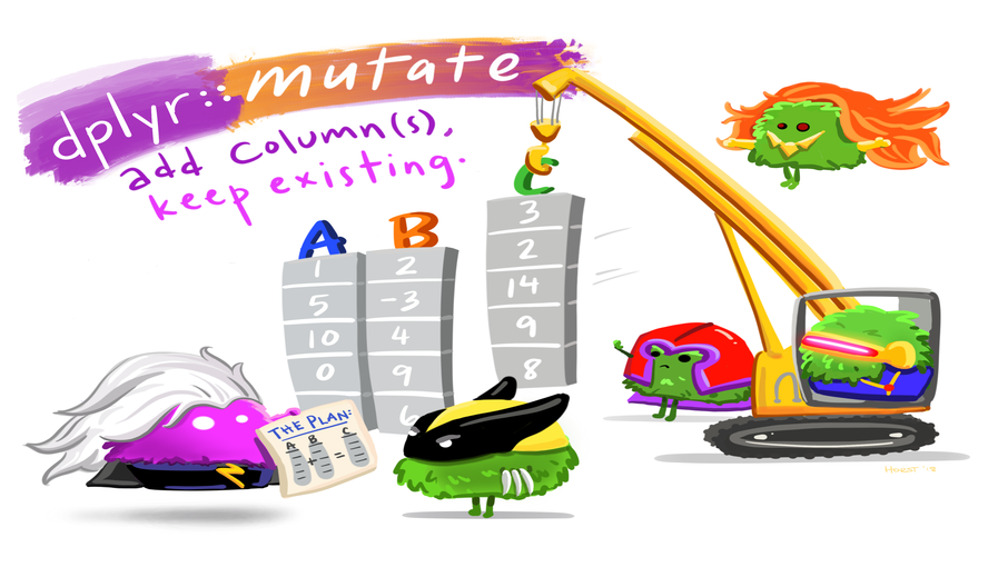

Within one mutate statement

Instant availability

Use new variables in the same function call right away!

judgments |>
  mutate(
    mood_change = mood_post - mood_pre,
    # remove missing data before computation
    mood_change_norm =
      abs(mood_change / mean(mood_change, na.rm = TRUE))) |>
  relocate(starts_with("mood")) |> 
  arrange(desc(mood_change_norm))

# A tibble: 188 × 160
   mood_pre mood_post mood_change mood_change_norm
      <dbl>     <dbl>       <dbl>            <dbl>
 1       66         0         -66             9.12
 2       77        22         -55             7.60
 3       47       100          53             7.32
 4       25        72          47             6.49
 5       22        69          47             6.49
 6       37        83          46             6.36
 7       20        62          42             5.80
 8       60       100          40             5.53
 9       22        60          38             5.25
10       30        68          38             5.25
# ℹ 178 more rows
# ℹ 156 more variables: start_date <chr>,
#   end_date <chr>, finished <dbl>,
#   condition <chr>, subject <dbl>, gender <chr>,
#   age <dbl>, STAI_pre_1_1 <dbl>,
#   STAI_pre_1_2 <dbl>, STAI_pre_1_3 <dbl>,
#   STAI_pre_1_4 <dbl>, STAI_pre_1_5 <dbl>, …

Replacing columns

Update

Using existing columns updates their content.

Warning

If not using names actions are used as names (avoid)

`mutate()` existing columns, centering `mood` columns

judgments |>
  mutate(mood_pre = mood_pre / mean(mood_pre, na.rm = TRUE),
         mood_post = mood_post / mean(mood_post, na.rm = TRUE),
         mood_pre / mean(mood_post, na.rm = TRUE)) |> 
  select(starts_with("mood"))

# A tibble: 188 × 3
   mood_pre mood_post mood_pre/mean(mood_post, n…¹
      <dbl>     <dbl>                        <dbl>
 1    1.36     NA                            1.36 
 2    0.994     0.680                        0.994
 3    0.371     0.971                        0.371
 4    0.893     1.10                         0.893
 5    0.809    NA                            0.809
 6    1.23      1.18                         1.23 
 7   NA        NA                           NA    
 8    1.68     NA                            1.68 
 9    1.13      1.20                         1.13 
10    0.505     1.10                         0.505
# ℹ 178 more rows
# ℹ abbreviated name:
#   ¹`mood_pre/mean(mood_post, na.rm = TRUE)`

Vectorised if_else

Categorize values based on one condition.
TRUE/FALSE expression
Additionally: missing values can have its own category.

judgments |> 
  mutate(
   mood_pre_cat = if_else(mood_pre < 25, "poor", "other", missing = "unknown")
         ) |> 
  select(mood_pre, mood_pre_cat)

# A tibble: 188 × 2
   mood_pre mood_pre_cat
      <dbl> <chr>       
 1       81 other       
 2       59 other       
 3       22 poor        
 4       53 other       
 5       48 other       
 6       73 other       
 7       NA unknown     
 8      100 other       
 9       67 other       
10       30 other       
# ℹ 178 more rows

Switch statements `case_when()` and `case_match()`

Categorize mood_pre. Tests come sequentially

judgments |>
  mutate(mood_pre_cat = case_when(
    mood_pre < 25   ~ "poor", 
    mood_pre < 50   ~ "mid", 
    mood_pre < 75   ~ "great",
    mood_pre <= 100 ~ "exceptional",
    TRUE ~ "missing data")) |> 
  select(mood_pre, mood_pre_cat) #|>

# A tibble: 188 × 2
   mood_pre mood_pre_cat
      <dbl> <chr>       
 1       81 exceptional 
 2       59 great       
 3       22 poor        
 4       53 great       
 5       48 mid         
 6       73 great       
 7       NA missing data
 8      100 exceptional 
 9       67 great       
10       30 mid         
# ℹ 178 more rows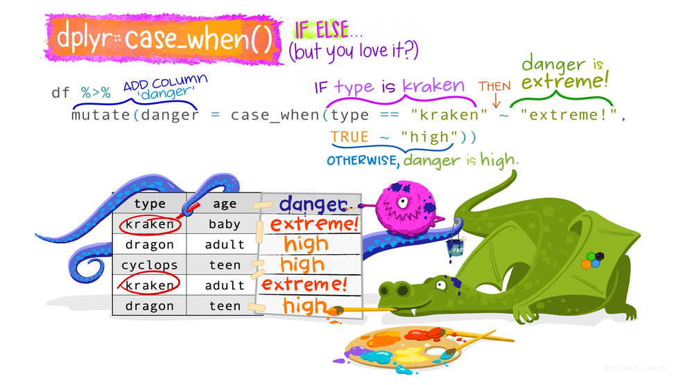

 # count(mood_pre_cat)

Note

The function if_else() provides a short hand for the case of a single condition only.

`case_match()` version

The column is stated only once.
.default to control the unmatched values
New in dplyr 1.1.0

judgments |>
  mutate(mood_pre_cat = case_match(
    mood_pre,
    c(0:24)   ~ "poor", 
    c(25:49)  ~ "mid", 
    c(50:74)  ~ "great",
    c(75:100) ~ "exceptional",
    .default = "missing data")) |> 
  select(mood_pre, mood_pre_cat)

# A tibble: 188 × 2
   mood_pre mood_pre_cat
      <dbl> <chr>       
 1       81 exceptional 
 2       59 great       
 3       22 poor        
 4       53 great       
 5       48 mid         
 6       73 great       
 7       NA missing data
 8      100 exceptional 
 9       67 great       
10       30 mid         
# ℹ 178 more rows

Act on multiple columns at once using `across()`

Usage

Can be plugged into mutate(), summarise()…

across(ON WHO, DO WHAT)

Columns selection:
- Argument .cols
- tidyselect helpers
- everything() = all columns.
- Conditions (boolean) needs where(), across(where(is.numeric))
Actions using functions:
- Argument .fns
- fun, arg1, arg2
- \(x) fun(x), with placeholder x
- Multiple functions as arguments need to be wrapped up
- New column names can be controlled

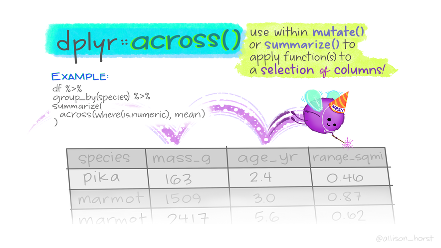
Examples of `across()` usage

Add 1 to the STAI questionnaire data

To convert Likert scales 0-4 to 1-5 (same column names)

judgments |> 
  mutate(across(contains("STAI"), `+`, 1)) |>
  select(starts_with("STAI"))

# A tibble: 188 × 42
   STAI_pre_1_1 STAI_pre_1_2 STAI_pre_1_3
          <dbl>        <dbl>        <dbl>
 1            3            2            3
 2            4            3            4
 3            5            4            4
 4            3            3            3
 5            2            2            2
 6            3            3            2
 7            3            3            2
 8            2            2            2
 9            3            3            2
10            5            3            4
# ℹ 178 more rows
# ℹ 39 more variables: STAI_pre_1_4 <dbl>,
#   STAI_pre_1_5 <dbl>, STAI_pre_1_6 <dbl>,
#   STAI_pre_1_7 <dbl>, STAI_pre_2_1 <dbl>,
#   STAI_pre_2_2 <dbl>, STAI_pre_2_3 <dbl>,
#   STAI_pre_2_4 <dbl>, STAI_pre_2_5 <dbl>,
#   STAI_pre_2_6 <dbl>, STAI_pre_2_7 <dbl>, …

To specify different names and not overwrite cols

judgments |> 
  mutate(across(starts_with("mood"), scale, 
                .names = "rescale_{.col}")) |>
  select(contains("mood"))

# A tibble: 188 × 4
   mood_pre mood_post rescale_mood_pre[,1]
      <dbl>     <dbl>                <dbl>
 1       81        NA               1.17  
 2       59        42              -0.0193
 3       22        60              -2.01  
 4       53        68              -0.343 
 5       48        NA              -0.612 
 6       73        73               0.735 
 7       NA        NA              NA     
 8      100        NA               2.19  
 9       67        74               0.412 
10       30        68              -1.58  
# ℹ 178 more rows
# ℹ 1 more variable: rescale_mood_post <dbl[,1]>

For `filter` the across is renamed to if any or all

Find rows where ANY of mood data columns are missing

judgments |> 
  filter(if_any(starts_with("mood_p"), is.na)) |>  #<<
  select(subject, starts_with("mood"))

# A tibble: 91 × 3
   subject mood_pre mood_post
     <dbl>    <dbl>     <dbl>
 1       2       81        NA
 2       7       48        NA
 3       5       NA        NA
 4       9      100        NA
 5      12       67        NA
 6      11       61        NA
 7      10       72        NA
 8       8       59        NA
 9      23       78        NA
10      21       68        NA
# ℹ 81 more rows

Find rows where BOTH of mood data columns are missing

judgments |> 
  filter(if_all(starts_with("mood_p"), is.na)) |> #<<
  select(subject, starts_with("mood"))

# A tibble: 1 × 3
  subject mood_pre mood_post
    <dbl>    <dbl>     <dbl>
1       5       NA        NA

Using lambdas

Reminder

\(x) x + 1 is just a shorthand for

function(x) {x + 1}

Add 1 to the STAI questionnaire data

judgments |> 
  mutate(across(contains("STAI"), 
                \(x) x + 1)) |>
  select(starts_with("STAI"))

# A tibble: 188 × 42
   STAI_pre_1_1 STAI_pre_1_2 STAI_pre_1_3
          <dbl>        <dbl>        <dbl>
 1            3            2            3
 2            4            3            4
 3            5            4            4
 4            3            3            3
 5            2            2            2
 6            3            3            2
 7            3            3            2
 8            2            2            2
 9            3            3            2
10            5            3            4
# ℹ 178 more rows
# ℹ 39 more variables: STAI_pre_1_4 <dbl>,
#   STAI_pre_1_5 <dbl>, STAI_pre_1_6 <dbl>,
#   STAI_pre_1_7 <dbl>, STAI_pre_2_1 <dbl>,
#   STAI_pre_2_2 <dbl>, STAI_pre_2_3 <dbl>,
#   STAI_pre_2_4 <dbl>, STAI_pre_2_5 <dbl>,
#   STAI_pre_2_6 <dbl>, STAI_pre_2_7 <dbl>, …

Selecting columns with a predicate `where()`

Add 1 to numeric columns for all questionnaire data

Predicate means return TRUE or FALSE

judgments |> 
  mutate(across(where(is.numeric),
                \(x) x + 1))

# A tibble: 188 × 158
   start_date end_date  finished condition subject
   <chr>      <chr>        <dbl> <chr>       <dbl>
 1 11/3/2014  11/3/2014        2 control         3
 2 11/3/2014  11/3/2014        2 stress          2
 3 11/3/2014  11/3/2014        2 stress          4
 4 11/3/2014  11/3/2014        2 stress          5
 5 11/3/2014  11/3/2014        2 control         8
 6 11/3/2014  11/3/2014        2 stress          7
 7 11/3/2014  11/3/2014        2 control         6
 8 11/3/2014  11/3/2014        2 control        10
 9 11/3/2014  11/3/2014        2 stress         17
10 11/3/2014  11/3/2014        2 stress         14
# ℹ 178 more rows
# ℹ 153 more variables: gender <chr>, age <dbl>,
#   mood_pre <dbl>, mood_post <dbl>,
#   STAI_pre_1_1 <dbl>, STAI_pre_1_2 <dbl>,
#   STAI_pre_1_3 <dbl>, STAI_pre_1_4 <dbl>,
#   STAI_pre_1_5 <dbl>, STAI_pre_1_6 <dbl>,
#   STAI_pre_1_7 <dbl>, STAI_pre_2_1 <dbl>, …

Watch out

Now we also get subject changed!

Tip

However, .grouped variable are protected

group_by(judgments, subject) |>
  mutate(across(where(is.numeric), 
                \(x) x + 1)) |>
  select(finished, subject) |> 
  head(3L) |> 
  knitr::kable()

finished	subject
2	2
2	1
2	3

More advanced across(): multiple functions

Summarise by the mean of mood

summarise(judgments,
          across(starts_with("mood"), 
                 list(mean, sd), na.rm = TRUE))

# A tibble: 1 × 4
  mood_pre_1 mood_pre_2 mood_post_1 mood_post_2
       <dbl>      <dbl>       <dbl>       <dbl>
1       59.4       18.6        61.8        20.5

Remember what was done in the guided practical datasauRus

Better with naming and function arguments

summarise(judgments,
          across(starts_with("moral_dil"), 
                 list(aveg = \(x) mean(x, na.rm = TRUE), 
                      sdev = \(x) sd(x, na.rm = TRUE))))

# A tibble: 1 × 14
  moral_dilemma_dog_aveg moral_dilemma_dog_sdev
                   <dbl>                  <dbl>
1                   7.35                   2.17
# ℹ 12 more variables:
#   moral_dilemma_wallet_aveg <dbl>,
#   moral_dilemma_wallet_sdev <dbl>,
#   moral_dilemma_plane_aveg <dbl>,
#   moral_dilemma_plane_sdev <dbl>,
#   moral_dilemma_resume_aveg <dbl>,
#   moral_dilemma_resume_sdev <dbl>, …

Manipulation by row

Summing all scores for the STAI questionnaire

judgments |> 
  mutate(total_stai = 
           sum(across(contains("STAI")), 
               na.rm = TRUE)) |>
  select(subject, total_stai, contains("STAI"))

# A tibble: 188 × 44
   subject total_stai STAI_pre_1_1 STAI_pre_1_2
     <dbl>      <dbl>        <dbl>        <dbl>
 1       2      22866            2            1
 2       1      22866            3            2
 3       3      22866            4            3
 4       4      22866            2            2
 5       7      22866            1            1
 6       6      22866            2            2
 7       5      22866            2            2
 8       9      22866            1            1
 9      16      22866            2            2
10      13      22866            4            2
# ℹ 178 more rows
# ℹ 40 more variables: STAI_pre_1_3 <dbl>,
#   STAI_pre_1_4 <dbl>, STAI_pre_1_5 <dbl>,
#   STAI_pre_1_6 <dbl>, STAI_pre_1_7 <dbl>,
#   STAI_pre_2_1 <dbl>, STAI_pre_2_2 <dbl>,
#   STAI_pre_2_3 <dbl>, STAI_pre_2_4 <dbl>,
#   STAI_pre_2_5 <dbl>, STAI_pre_2_6 <dbl>, …

Tip

rowwise() - computation by row
c_across() - selects columns with tidyselect

judgments |>
  rowwise() |> #<<
  mutate(total_stai = sum(c_across( #<<
    starts_with("STAI")), na.rm = TRUE)) |>
  select(subject, total_stai, contains("STAI"))

# A tibble: 188 × 44
# Rowwise: 
   subject total_stai STAI_pre_1_1 STAI_pre_1_2
     <dbl>      <dbl>        <dbl>        <dbl>
 1       2         64            2            1
 2       1        200            3            2
 3       3        212            4            3
 4       4        148            2            2
 5       7         66            1            1
 6       6        134            2            2
 7       5         64            2            2
 8       9         42            1            1
 9      16        122            2            2
10      13        196            4            2
# ℹ 178 more rows
# ℹ 40 more variables: STAI_pre_1_3 <dbl>,
#   STAI_pre_1_4 <dbl>, STAI_pre_1_5 <dbl>,
#   STAI_pre_1_6 <dbl>, STAI_pre_1_7 <dbl>,
#   STAI_pre_2_1 <dbl>, STAI_pre_2_2 <dbl>,
#   STAI_pre_2_3 <dbl>, STAI_pre_2_4 <dbl>,
#   STAI_pre_2_5 <dbl>, STAI_pre_2_6 <dbl>, …

Your turn!

Exercises

Abbreviate the gender column such that only the first character remains
Create a new STAI_pre_category column. Use case_match() to categorize values in STAI_pre as “low”, “normal” or “high”. For values < 25 in STAI_pre assign “low”, for values > 65 assign “high”, and for all other values assign “normal”.

Hint: To easily see the new column, use relocate() to move it to the first position of the dataframe.

10:00

Solution

judgments |> 
  mutate(gender = str_sub(gender, 1,1))

# A tibble: 188 × 158
   start_date end_date  finished condition subject
   <chr>      <chr>        <dbl> <chr>       <dbl>
 1 11/3/2014  11/3/2014        1 control         2
 2 11/3/2014  11/3/2014        1 stress          1
 3 11/3/2014  11/3/2014        1 stress          3
 4 11/3/2014  11/3/2014        1 stress          4
 5 11/3/2014  11/3/2014        1 control         7
 6 11/3/2014  11/3/2014        1 stress          6
 7 11/3/2014  11/3/2014        1 control         5
 8 11/3/2014  11/3/2014        1 control         9
 9 11/3/2014  11/3/2014        1 stress         16
10 11/3/2014  11/3/2014        1 stress         13
# ℹ 178 more rows
# ℹ 153 more variables: gender <chr>, age <dbl>,
#   mood_pre <dbl>, mood_post <dbl>,
#   STAI_pre_1_1 <dbl>, STAI_pre_1_2 <dbl>,
#   STAI_pre_1_3 <dbl>, STAI_pre_1_4 <dbl>,
#   STAI_pre_1_5 <dbl>, STAI_pre_1_6 <dbl>,
#   STAI_pre_1_7 <dbl>, STAI_pre_2_1 <dbl>, …

judgments |>
  mutate(STAI_pre_category = case_match(
    STAI_pre, 
    c(0:24)  ~ "low",
    c(25:65) ~ "normal",
    .default = "high")) |>
  relocate(STAI_pre_category)

# A tibble: 188 × 159
   STAI_pre_category start_date end_date  finished
   <chr>             <chr>      <chr>        <dbl>
 1 normal            11/3/2014  11/3/2014        1
 2 normal            11/3/2014  11/3/2014        1
 3 normal            11/3/2014  11/3/2014        1
 4 normal            11/3/2014  11/3/2014        1
 5 normal            11/3/2014  11/3/2014        1
 6 normal            11/3/2014  11/3/2014        1
 7 normal            11/3/2014  11/3/2014        1
 8 low               11/3/2014  11/3/2014        1
 9 normal            11/3/2014  11/3/2014        1
10 normal            11/3/2014  11/3/2014        1
# ℹ 178 more rows
# ℹ 155 more variables: condition <chr>,
#   subject <dbl>, gender <chr>, age <dbl>,
#   mood_pre <dbl>, mood_post <dbl>,
#   STAI_pre_1_1 <dbl>, STAI_pre_1_2 <dbl>,
#   STAI_pre_1_3 <dbl>, STAI_pre_1_4 <dbl>,
#   STAI_pre_1_5 <dbl>, STAI_pre_1_6 <dbl>, …

Solution

judgments |> 
  mutate(across(contains("REI"), 
                \(x) x / 5)) |>
  relocate(contains("REI"))

# A tibble: 188 × 158
   REI_1 REI_2 REI_3 REI_4 REI_5 REI_6 REI_7 REI_8
   <dbl> <dbl> <dbl> <dbl> <dbl> <dbl> <dbl> <dbl>
 1   1     0.8   1     0.8   0.8   1     0.6   0.8
 2  NA    NA    NA    NA    NA    NA    NA    NA  
 3  NA    NA    NA    NA    NA    NA    NA    NA  
 4  NA    NA    NA    NA    NA    NA    NA    NA  
 5   0.6   0.6   0.6   0.6   0.8   0.6   0.6   0.6
 6  NA    NA    NA    NA    NA    NA    NA    NA  
 7   0.8   0.8   0.8   0.8   0.8   0.8   0.6   0.8
 8   0.8   1     1     1     1     1     1     1  
 9  NA    NA    NA    NA    NA    NA    NA    NA  
10  NA    NA    NA    NA    NA    NA    NA    NA  
# ℹ 178 more rows
# ℹ 150 more variables: REI_9 <dbl>,
#   REI_10 <dbl>, REI_11 <dbl>, REI_12 <dbl>,
#   REI_13 <dbl>, REI_14 <dbl>, REI_15 <dbl>,
#   REI_16 <dbl>, REI_17 <dbl>, REI_18 <dbl>,
#   REI_19 <dbl>, REI_20 <dbl>, REI_21 <dbl>,
#   REI_22 <dbl>, REI_23 <dbl>, REI_24 <dbl>, …

Next up!

Grouping and summarising with dplyr

Data wrangling - Introduction

Introduction

This lecture

dplyr Introduction: Cheat sheets

Using the dplyr package

Preparing the data

Your turn!

Inspecting tibbles

Inspect tibbles with glimpse()

Selecting columns

Reminder tidyselect

Combining helpers

Selecting with quoted names

Helpers are evaluated from left to right

Selecting columns

relocate()

Filtering for rows: filter()

Filtering rows

Multiple conditions: AND

Multiple conditions: OR

Filtering out rows

Filter rows, helper between()

Set operations with filter()

Filter out rows that are unique: distinct()

Do we have different start / end dates?

Use distinct() to remove duplicated rows:

Sort columns: arrange()

A nested sorting example

Reverse sort columns

Verbs to inspect data

Summary

Your turn!

Exercises

Solution

Solution

Transforming columns

Changing column names

rename(data, new_name = old_name)

With a function: rename_with()

Adding columns: mutate()

Within one mutate statement

Replacing columns

mutate() existing columns, centering mood columns

Vectorised if_else

Switch statements case_when() and case_match()

case_match() version

Act on multiple columns at once using across()

Examples of across() usage

Add 1 to the STAI questionnaire data

To specify different names and not overwrite cols

For filter the across is renamed to if any or all

Find rows where ANY of mood data columns are missing

Find rows where BOTH of mood data columns are missing

Using lambdas

Add 1 to the STAI questionnaire data

Selecting columns with a predicate where()

Add 1 to numeric columns for all questionnaire data

More advanced across(): multiple functions

Summarise by the mean of mood

Better with naming and function arguments

Manipulation by row

Summing all scores for the STAI questionnaire

Your turn!

Exercises

Solution

Solution

Next up!

`dplyr` Introduction: Cheat sheets

Using the `dplyr` package

Inspect tibbles with `glimpse()`

Reminder `tidyselect`

`relocate()`

Filtering for rows: `filter()`

Filter rows, helper `between()`

Set operations with `filter()`

Filter out rows that are unique: `distinct()`

Use `distinct()` to remove duplicated rows:

Sort columns: `arrange()`

`rename(data, new_name = old_name)`

With a function: `rename_with()`

Adding columns: `mutate()`

`mutate()` existing columns, centering `mood` columns

Switch statements `case_when()` and `case_match()`

`case_match()` version

Act on multiple columns at once using `across()`

Examples of `across()` usage

For `filter` the across is renamed to if any or all

Selecting columns with a predicate `where()`