Plotting data

ggplot, part 2

Roland Krause

Rworkshop

Thursday, 8 February 2024

Introduction

More ggplot2!

Scales catalogue

Scales for all

62 functions available!

Functions are based on this scheme:

scale_{aes}_{type}()

Arguments to change default

breaks, choose where are labels
labels, usually with package scales
trans, to change to i.e log

tidyr `crossing` + glue `glue_data` trick

To generate all combinations

tidyr::crossing(aes = c("fill", "colour", "alpha", "x", "y"),
         type = c("continuous", "discrete", "date")) |>
  glue::glue_data("scale_{aes}_{type}()")

scale_alpha_continuous()
scale_alpha_date()
scale_alpha_discrete()
scale_colour_continuous()
scale_colour_date()
scale_colour_discrete()
scale_fill_continuous()
scale_fill_date()
scale_fill_discrete()
scale_x_continuous()
scale_x_date()
scale_x_discrete()
scale_y_continuous()
scale_y_date()
scale_y_discrete()

scales::label_percent()(c(0.4, 0.6, .95))

[1] "40%" "60%" "95%"

scales::label_comma()(20^(1:4))

[1] "20"      "400"     "8,000"   "160,000"

scales::breaks_log()(20^(1:3))

[1]    10    30   100   300  1000  3000 10000

Scales

Scales transformation

Starwars: who is the massive guy?

ggplot(starwars, aes(x = height, y = mass)) +
  geom_point(size = 2) # from dplyr

ggplot(starwars, aes(x = height, y = mass)) +
  geom_point(alpha = 0.6, size = 2) +
  geom_text(data = \(x) filter(x, mass > 1000),
            aes(label = name), nudge_y = -0.2) +
  annotation_logticks(sides = "l") +
  scale_y_continuous(trans = "pseudo_log")

pseudo_log is available through scales.

All geometries geom_ can take either a data.frame or a function, here geom_text().

Native lambda, < 4.1 would be function(x) filter(x, mass > 1000).

Colors

Custom colors

Better: see Emil Hvitfeldt repo

Changing colours for categories

Default is `scale_fill_hue()`

filter(starwars, !is.na(gender)) |>
ggplot(aes(y = gender,
          fill = fct_lump_n(species, 8) |>
                 fct_infreq())) +
  geom_bar(position = "fill") +
  scale_fill_hue() +
  labs(fill = "top 8 Species\n(ranked)")

Rbrewer is a safe alternative

filter(starwars, !is.na(gender)) |>
ggplot(aes(y = gender,
          fill = fct_lump_n(species, 8) |>
                 fct_infreq())) +
  geom_bar(position = "fill") +
  scale_fill_brewer(palette = "Set1") +
  labs(fill = "top 8 Species\n(ranked)")

Predefined colour palettes

library(RColorBrewer)
par(mar = c(0, 4, 
            0, 0))
display.brewer.all()

Colour gradient, for continuous variables

The default gradient generated by ggplot2 is not very good… Better off using viridis (scale_color_viridis_c() c for continuous)

penguins |>
  ggplot(aes(x = bill_length_mm, 
             y = bill_depth_mm, 
             colour = body_mass_g)) +
  geom_point(alpha = 0.6, size = 5)

penguins |>
  ggplot(aes(x = bill_length_mm, y = bill_depth_mm, 
             colour = body_mass_g)) +
  geom_point(alpha = 0.6, size = 5) +
  scale_color_viridis_c()

Viridis palettes

5 different scales
Also for discrete variables
viridis is colour blind friendly and nice in b&w
In ggplot2 since v3.0 but no the default

penguins |>
  ggplot(aes(x = bill_length_mm, y = bill_depth_mm, 
             colour = species)) +
  geom_point(alpha = 0.6, size = 5) +
  scale_color_viridis_d()

Binning instead of gradient

Binning help grouping observations

Default blue gradient, viridis option
Number of bins, limits can be changed

penguins |>
  ggplot(aes(x = bill_length_mm, y = bill_depth_mm, 
             colour = body_mass_g)) +
  geom_point(alpha = 0.6, size = 5) +
  scale_color_binned(type = "viridis")

Merge similar guides

Size & colour on same variable ➡️ 2 guides

penguins |>
  ggplot(aes(x = bill_length_mm, y = bill_depth_mm, 
             colour = body_mass_g,
             size = body_mass_g)) +
  geom_point(alpha = 0.6) +
  scale_color_viridis_c()

`guides()` merge both aesthetics

penguins |>
  ggplot(aes(x = bill_length_mm, y = bill_depth_mm, 
             colour = body_mass_g, size = body_mass_g)) +
  geom_point(alpha = 0.6) +
  scale_color_viridis_c() +
  guides(colour = "legend")

Facets: `facet_wrap()`

Easiest way: facet_wrap()
Use a formula (in R ~)
facet_wrap() is for one var
Or the vars() function

ggplot(penguins, 
       aes(bill_depth_mm, 
           bill_length_mm)) +
  geom_point() +
  facet_wrap(~ species)

Facets layout

Specify the number of rows/columns:

ncol = integer
nrow = integer

fc <- ggplot(penguins, 
       aes(bill_depth_mm, 
           bill_length_mm)) +
  geom_point()
fc + facet_wrap(~ species, ncol = 2)

Facets, free scales

⚠️ Make comparison harder

x or y (free_x / free_y)

fc + facet_wrap(~ species, scales = "free_y")

Both axis

fc + facet_wrap(~ species, scales = "free")

`facet_grid()` to lay out panels in a grid

Specify a 2 sides formula

rows on the left, columns on the right separated by a tilde ~

ggplot(penguins, 
       aes(bill_depth_mm, 
           bill_length_mm)) +
  geom_point() +
  facet_grid(island ~ species)

Barplots in facets

facet_grid() can also be used with one variable, complemented by a placeholder: .

Waste of space

ggplot(starwars) +
  geom_bar(aes(y = gender, fill = sex)) +
  facet_grid(fct_lump_min(species, 4) ~ .) +
  labs(y = NULL)

Optimize by removing empty slots

ggplot(starwars) +
  geom_bar(aes(y = gender, fill = sex)) +
  facet_grid(fct_lump_min(species, 4) ~ .,
             space = "free", scales = "free_y") +
  labs(y = NULL)

Extensions

ggplot2 introduced the possibility for the community to create extensions, they are referenced on a dedicated site

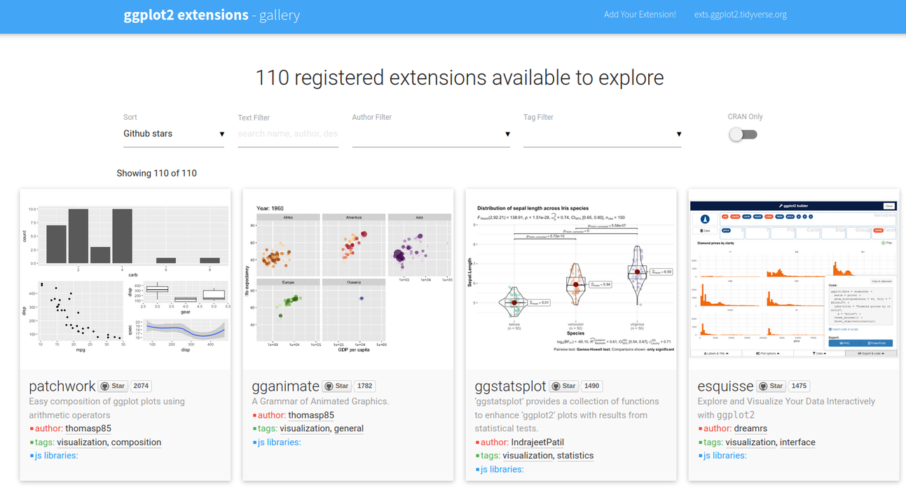
(https://exts.ggplot2.tidyverse.org/gallery/)

Fancy nested facets using `ggh4x`, code by Eric Koncina

library(ggh4x)
library(ggtext)

strip_ektheme <- strip_nested(
  text_x = distribute_args(
    size = c(14, 10), colour = c("darkred", "black"), 
    face = c("bold", "plain"),
    fill = list(NA, "lightblue"),
    box.color = list(NA, "darkblue"),
    halign = list(0.5, 0.5), valign = list(1, 0.5),
    linetype = list(0, 1), r = list(NULL, unit(5, "pt")),
    width = list(NULL, unit(1, "npc")),
    padding = list(NULL, margin(5, 0, 4, 0)),
    margin = list(margin(1, 0, 2, 0), margin(7, 3, 3, 3)),
    .fun = element_textbox),
  size = "variable",
  by_layer_x = TRUE
)
pivot_longer(penguins, names_to = c("what", "measure"),
             values_to = "value", 
             bill_length_mm:body_mass_g, names_sep = "_") |> 
  ggplot(aes(x = species, y = log(value))) +
  geom_violin(trim = FALSE) +
  facet_nested(~ what + measure, strip = strip_ektheme, #<<
               nest_line = TRUE, resect = unit(15, "mm"), #<<
               axes = TRUE, remove_labels = TRUE) + #<<
  theme_classic(14) +
  theme(strip.background = element_blank(), 
        axis.text.x = element_text(angle = 45, hjust = 1),
        ggh4x.facet.nestline = element_line(colour = "rosybrown")) #<<

Cosmetics 💅

Black theme

Using Bob Rudis `hrbrthemes` package

library(hrbrthemes)
ggplot(penguins,
       aes(x = bill_length_mm,
           y = bill_depth_mm,
           colour = species)) +
  geom_point() +
  geom_smooth(method = "lm", formula = 'y ~ x',
      # no standard error ribbon
              se = FALSE) +
  facet_grid(island ~ .) +
  labs(x = "length (mm)", y = "depth (mm)",
       title = "Palmer penguins",
       subtitle = "bill dimensions over location and species",
       caption = "source: Horst AM, Hill AP, Gorman KB (2020)") +
  # hrbrthemes specifications
  scale_fill_ipsum() +
  theme_ft_rc(14) +
  # tweak the theme
  theme(panel.grid.major.y = element_blank(),
   panel.grid.major.x = element_line(size = 0.5),
   plot.caption = element_text(face = "italic"),
   strip.text = element_text(face = "bold"),
   plot.caption.position = "plot")

Compose plots with `patchwork`

Patchwork is developed by Thomas Lin Pedersen, main maintainer of `ggplot2`.

Define 3 plots and assign them names

p1 <- ggplot(penguins, 
             aes(x = species)) +
  geom_bar() +
  labs(title = "Species distribution")
p2 <- ggplot(penguins, 
             aes(y = island)) +
  geom_bar() +
  labs(title = "Island but flipped")
p3 <- ggplot(penguins, 
             aes(x = body_mass_g,
                 y = bill_depth_mm,
                 colour = sex)) +
  geom_point()
p1

p2

p3

Now, compose them!

Compose plots with `patchwork`

`patchwork` provides an API using the classic arithmetic operators

library(patchwork)
(( p1 | p2 ) / p3) +
  # add tags and main title
  plot_annotation(tag_levels = 'A',
                  title = 'Plots about penguins') &
  # modify all plots recursively
  theme_minimal() +
  theme(text = element_text('Roboto'))

Polished example by Cédric Scherer

Using patchwork, ggforce T. Pedersen and ggtext Claus O. Wilke

Text paths, curved labels in data

library(geomtextpath)
ggplot(penguins,
       aes(x = bill_length_mm, y = bill_depth_mm, colour = species)) +
  geom_point(alpha = 0.3) +
  stat_ellipse(aes(label = species),
    geom = "textpath", hjust = c(0.55)) +
  theme_bw(14) + theme(legend.position = "none")

ggplot(penguins,
       aes(x = bill_length_mm / bill_depth_mm, 
           colour = species)) +
  stat_density(aes(label = species),
    geom = "textpath", hjust = c(0.25)) +
  theme_bw(14) + theme(legend.position = "none")

Exporting, interactive or passive mode

Right panel

Using the Export button in the Plots panel

ggsave

Save the ggplot object, 2nd argument, here p or last_plot()
Guesses the output type by the extension (jpg, png, pdf etc.)

ggsave("my_name.png", p, width = 60, height = 30, units = "mm")
ggsave("my_name.pdf", last_plot(), width = 50, height = 50, units = "mm")

Quarto documents

If needed, adjust the chunk options:
- Size: fig.height, fig.width
- Ratio: fig.asp…

Plot your data!

Warning

Never trust summary statistics alone; always visualize your data

— Alberto Cairo

Missing features

Geoms list here

geom_tile() heatmap
geom_bind2d() 2D binning
geom_abline() slope

Stats list here

stat_ellipse() (ggforge seen)
stat_summary() easy mean, 95CI etc.

Plot on multi-pages

ggforce::facet_grid_paginate() facets
gridExtra::marrangeGrob() plots

Coordinate / transform

coord_cartesian() for zooming in

Customise theme elements

Legend & guide tweaks
Major/minor grids
Font, faces
Margins
Labels & ticks
Strip positions
See live examples of pre-built themes

Build your plot with point and click

Using `esquisse` Rstudio addin by dreamRs

Before we stop

You learned to:

Apprehend facets
Color schemes and gradients
Discover extensions
The endless potential of cosmetic improvements

Acknowledgments

Thomas Lin Pedersen, great webinar Plotting everything with ggplot2:
- part 1, ggplot2 API
- part 2, extending ggplot2
Bob Rudis
Allison M. Horst, Alison P. Hill and Kristen B. Gorman *
DreamRs (Victor Perrier, Fanny Meyer)
Claus O. Wilke
Hadley Wickham
Cédric Scherer

Further reading

ggplot2 book by H. Wickham (free access)
NEW official FAQ, axes, facets, custom, annot, reorder, bars
R for Data Science by H. Wickham / G. Gromelund (free access)
TidyTuesday challenges
Vizualisation gallery by Cédric Scherer
plotting tutorial by Cédric Scherer

Thank you for your attention!

*: Palmer penguins, data are available by CC-0 license and Artwork by Allison Horst

Plotting data

Introduction

More ggplot2!

Scales catalogue

Scales for all

62 functions available!

Arguments to change default

tidyr crossing + glue glue_data trick

Scales

Scales transformation

Starwars: who is the massive guy?

Colors

Custom colors

Changing colours for categories

Default is scale_fill_hue()

Rbrewer is a safe alternative

Predefined colour palettes

Colour gradient, for continuous variables

Viridis palettes

Binning instead of gradient

Binning help grouping observations

Merge similar guides

Size & colour on same variable ➡️ 2 guides

guides() merge both aesthetics

Facets

Facets: facet_wrap()

Creating facets

Facets layout

Specify the number of rows/columns:

Facets, free scales

⚠️ Make comparison harder

facet_grid() to lay out panels in a grid

Specify a 2 sides formula

Barplots in facets

Waste of space

Optimize by removing empty slots

Extensions

Fancy nested facets using ggh4x, code by Eric Koncina

Cosmetics 💅

Black theme

Using Bob Rudis hrbrthemes package

Compose plots with patchwork

Patchwork is developed by Thomas Lin Pedersen, main maintainer of ggplot2.

Define 3 plots and assign them names

Compose plots with patchwork

patchwork provides an API using the classic arithmetic operators

Polished example by Cédric Scherer

Text paths, curved labels in data

Exporting, interactive or passive mode

Right panel

ggsave

Quarto documents

Plot your data!

Missing features

Geoms list here

Stats list here

Plot on multi-pages

Coordinate / transform

Customise theme elements

Build your plot with point and click

Using esquisse Rstudio addin by dreamRs

Before we stop

Thank you for your attention!

tidyr `crossing` + glue `glue_data` trick

Default is `scale_fill_hue()`

`guides()` merge both aesthetics

Facets: `facet_wrap()`

`facet_grid()` to lay out panels in a grid

Fancy nested facets using `ggh4x`, code by Eric Koncina

Using Bob Rudis `hrbrthemes` package

Compose plots with `patchwork`

Patchwork is developed by Thomas Lin Pedersen, main maintainer of `ggplot2`.

Compose plots with `patchwork`

`patchwork` provides an API using the classic arithmetic operators

Using `esquisse` Rstudio addin by dreamRs