Joins and pivots

Merging data

Milena Zizovic/Roland Krause

Rworkshop

Tuesday, 11 February 2025

Introduction

Motivation

Joining data frames

How do we refer to a particular observation?

Primary key

The column that uniquely identifies an observation: - Frequently an ID - Can be introduced by row_number if no primary column exists bona fide observations

Composite key

Several columns that together identify an observation uniquely to serve as primary key.

Like patient and visit

Foreign key

A key referring to observations in another table

Your turn!

Tibbles do not have row names!

Frequently these are the primary keys! Use as_tibble(data, rownames = "ID") to make the rownames into a proper column.

Which columns are keys?

In judgments
In trees
In swiss

03:00

Solution

Primary key in `judgments`

select(judgments, subject)

# A tibble: 188 × 1
   subject
     <dbl>
 1       2
 2       1
 3       3
 4       4
 5       7
 6       6
 7       5
 8       9
 9      16
10      13
# ℹ 178 more rows

Solution - Trees

Composite key from all the variables

sample_n(trees, 5)

  Girth Height Volume
1  16.3     77   42.6
2  18.0     80   51.0
3  20.6     87   77.0
4  12.0     75   19.1
5  10.8     83   19.7

Or a primary key from row numbers

as_tibble(trees, 
          rownames = "ID")

# A tibble: 31 × 4
   ID    Girth Height Volume
   <chr> <dbl>  <dbl>  <dbl>
 1 1       8.3     70   10.3
 2 2       8.6     65   10.3
 3 3       8.8     63   10.2
 4 4      10.5     72   16.4
 5 5      10.7     81   18.8
 6 6      10.8     83   19.7
 7 7      11       66   15.6
 8 8      11       75   18.2
 9 9      11.1     80   22.6
10 10     11.2     75   19.9
# ℹ 21 more rows

Solution `swiss`

Province is primary key.

Once you took care of the rownames.

as_tibble(swiss, rownames = "Province")

# A tibble: 47 × 7
   Province     Fertility Agriculture Examination Education
   <chr>            <dbl>       <dbl>       <int>     <int>
 1 Courtelary        80.2        17            15        12
 2 Delemont          83.1        45.1           6         9
 3 Franches-Mnt      92.5        39.7           5         5
 4 Moutier           85.8        36.5          12         7
 5 Neuveville        76.9        43.5          17        15
 6 Porrentruy        76.1        35.3           9         7
 7 Broye             83.8        70.2          16         7
 8 Glane             92.4        67.8          14         8
 9 Gruyere           82.4        53.3          12         7
10 Sarine            82.9        45.2          16        13
# ℹ 37 more rows
# ℹ 2 more variables: Catholic <dbl>,
#   Infant.Mortality <dbl>

Mutating joins

Matching subjects in two tibbles

Additional data on coffee consumption

Manual input using tribble()

coffee_drinkers <- 
  tribble(~student, ~coffee_shots, 
          21,       1,
          23,       4,
          28,       2)

coffee_drinkers

# A tibble: 3 × 2
  student coffee_shots
    <dbl>        <dbl>
1      21            1
2      23            4
3      28            2

Smaller sample set

From judgements

subject_mood <- judgments |>
  select(subject, condition, gender, 
         starts_with("mood")) |> 
  distinct()
subject_mood

# A tibble: 187 × 5
   subject condition gender mood_pre mood_post
     <dbl> <chr>     <chr>     <dbl>     <dbl>
 1       2 control   female       81        NA
 2       1 stress    female       59        42
 3       3 stress    female       22        60
 4       4 stress    female       53        68
 5       7 control   female       48        NA
 6       6 stress    female       73        73
 7       5 control   female       NA        NA
 8       9 control   male        100        NA
 9      16 stress    female       67        74
10      13 stress    female       30        68
# ℹ 177 more rows

Combining the two tables

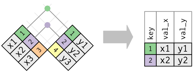
Inner join

Error! no common key.

inner_join(coffee_drinkers, 
           subject_mood)

Error in `inner_join()`:
! `by` must be supplied when `x` and `y` have no common variables.
ℹ Use `cross_join()` to perform a cross-join.

Provide the corresponding columns names

inner_join(subject_mood,
           coffee_drinkers, 
           by = join_by(subject == student))

# A tibble: 3 × 6
  subject condition gender mood_pre mood_post coffee_shots
    <dbl> <chr>     <chr>     <dbl>     <dbl>        <dbl>
1      23 control   female       78        NA            4
2      21 control   female       68        NA            1
3      28 stress    male         53        68            2

Mutating joins

Inner join

Creating new tables through joins

Key operations in data processing
Role of observations as row changes
inner_join() is the most strict join operations
merge is a similar operation in base R

Full Join

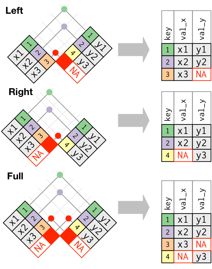
Example with `full_join()`

subject_mood |> 
  full_join(coffee_drinkers, 
             by = join_by(subject == student))

# A tibble: 187 × 6
   subject condition gender mood_pre mood_post coffee_shots
     <dbl> <chr>     <chr>     <dbl>     <dbl>        <dbl>
 1       2 control   female       81        NA           NA
 2       1 stress    female       59        42           NA
 3       3 stress    female       22        60           NA
 4       4 stress    female       53        68           NA
 5       7 control   female       48        NA           NA
 6       6 stress    female       73        73           NA
 7       5 control   female       NA        NA           NA
 8       9 control   male        100        NA           NA
 9      16 stress    female       67        74           NA
10      13 stress    female       30        68           NA
# ℹ 177 more rows

Two tables - same column names

What if we have gender in both tables?

coffee_drinkers <- mutate(coffee_drinkers, 
                          gender = c("female", "female", "male"))
coffee_drinkers

# A tibble: 3 × 3
  student coffee_shots gender
    <dbl>        <dbl> <chr> 
1      21            1 female
2      23            4 female
3      28            2 male

left_join(subject_mood,
          coffee_drinkers,
          by = join_by(subject == student))

# A tibble: 187 × 7
   subject condition gender.x mood_pre mood_post
     <dbl> <chr>     <chr>       <dbl>     <dbl>
 1       2 control   female         81        NA
 2       1 stress    female         59        42
 3       3 stress    female         22        60
 4       4 stress    female         53        68
 5       7 control   female         48        NA
 6       6 stress    female         73        73
 7       5 control   female         NA        NA
 8       9 control   male          100        NA
 9      16 stress    female         67        74
10      13 stress    female         30        68
# ℹ 177 more rows
# ℹ 2 more variables: coffee_shots <dbl>, gender.y <chr>

Need to disambiguate columns

Mutating joins distinguish the same column names by adding suffixes - .x and .y by default.

Two tables - same column names

Join by one column

right_join(subject_mood,
          coffee_drinkers,
          by = join_by(subject == student),
          suffix = c( "_mood", "_coffee"))

# A tibble: 3 × 7
  subject condition gender_mood mood_pre mood_post
    <dbl> <chr>     <chr>          <dbl>     <dbl>
1      23 control   female            78        NA
2      21 control   female            68        NA
3      28 stress    male              53        68
# ℹ 2 more variables: coffee_shots <dbl>,
#   gender_coffee <chr>

Controlling suffix names

Add suffix as additional parameter

Join by two columns

right_join(subject_mood,
          coffee_drinkers,
          by = join_by(subject == student, gender))

# A tibble: 3 × 6
  subject condition gender mood_pre mood_post coffee_shots
    <dbl> <chr>     <chr>     <dbl>     <dbl>        <dbl>
1      23 control   female       78        NA            4
2      21 control   female       68        NA            1
3      28 stress    male         53        68            2

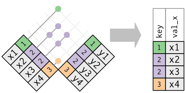
Filtering joins

Filtering joins -

`semi_join()`

Filter matches in x, no duplicates

`anti_join()`

Extract what does not match

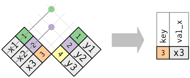
`semi_join()` to filter

Table x

key	x
1	x1
2	x2
3	x3
4	x4

Table y

key	y
1	y1
2	y2
2	y3
3	y4

Contains duplicated keys

There might be only a few cases…

Filtering

semi_join(tx, ty, 
          by = "key")

key	x
1	x1
2	x2
3	x3

Mutating join

inner_join(tx, ty, 
           by = "key")

key	x	y
1	x1	y1
2	x2	y2
2	x2	y3
3	x3	y4

Inequality joins

Redefine matches keys

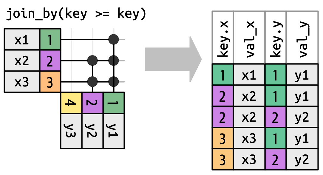
Caution

Unequal joins generate many additional rows.

Types of inqual joins

Cross joins match every pair of rows.
Inequality joins use <, <=, >, and >= instead of ==.
Rolling joins are similar to inequality joins but only find the closest match.
- Rolling joins allow to replace if/else or switch statements.
Overlap joins are a special type of inequality join designed to work with ranges.

Rewriting `case_when()`

Remember the tidyverse `switch`?

judgments |>
  mutate(mood_pre_cat = case_when(
    mood_pre < 25   ~ "poor", 
    mood_pre < 50   ~ "mid", 
    mood_pre < 75   ~ "great",
    mood_pre <= 100 ~ "exceptional",
    TRUE ~ "missing data")) |> 
  select(subject, mood_pre, mood_pre_cat)

# A tibble: 188 × 3
   subject mood_pre mood_pre_cat
     <dbl>    <dbl> <chr>       
 1       2       81 exceptional 
 2       1       59 great       
 3       3       22 poor        
 4       4       53 great       
 5       7       48 mid         
 6       6       73 great       
 7       5       NA missing data
 8       9      100 exceptional 
 9      16       67 great       
10      13       30 mid         
# ℹ 178 more rows

Rewriting `case_when()`

Remember the tidyverse `switch`?

judgments |>
  mutate(mood_pre_cat = case_when(
    mood_pre < 25   ~ "poor", 
    mood_pre < 50   ~ "mid", 
    mood_pre < 75   ~ "great",
    mood_pre <= 100 ~ "exceptional",
    TRUE ~ "missing data")) |> 
  select(subject, mood_pre, mood_pre_cat)

# A tibble: 188 × 3
   subject mood_pre mood_pre_cat
     <dbl>    <dbl> <chr>       
 1       2       81 exceptional 
 2       1       59 great       
 3       3       22 poor        
 4       4       53 great       
 5       7       48 mid         
 6       6       73 great       
 7       5       NA missing data
 8       9      100 exceptional 
 9      16       67 great       
10      13       30 mid         
# ℹ 178 more rows

Replacement

Replace with a table and a join

(mood_categories <- 
   tribble(
  ~score, ~label,
  25, "poor", 
  50, "mid", 
  75, "great",
 100, "exceptional",
 NA, "missing"))

# A tibble: 5 × 2
  score label      
  <dbl> <chr>      
1    25 poor       
2    50 mid        
3    75 great      
4   100 exceptional
5    NA missing

Join

left_join(subject_mood, mood_categories, 
          by = join_by(mood_pre < score), 
          keep = TRUE) |> 
  select(subject, mood_pre, score, label)

# A tibble: 394 × 4
   subject mood_pre score label      
     <dbl>    <dbl> <dbl> <chr>      
 1       2       81   100 exceptional
 2       1       59    75 great      
 3       1       59   100 exceptional
 4       3       22    25 poor       
 5       3       22    50 mid        
 6       3       22    75 great      
 7       3       22   100 exceptional
 8       4       53    75 great      
 9       4       53   100 exceptional
10       7       48    50 mid        
# ℹ 384 more rows

Not exactly helpful

Multiple entries (correctly) matching the condition.

Rolling join

Make it a rolling join with `closest()`

left_join(subject_mood, mood_categories, 
          by = join_by(
            closest(
              mood_pre <= score)), 
          keep = TRUE) |> 
  select(subject, mood_pre, score, label)

# A tibble: 187 × 4
   subject mood_pre score label      
     <dbl>    <dbl> <dbl> <chr>      
 1       2       81   100 exceptional
 2       1       59    75 great      
 3       3       22    25 poor       
 4       4       53    75 great      
 5       7       48    50 mid        
 6       6       73    75 great      
 7       5       NA    NA missing    
 8       9      100   100 exceptional
 9      16       67    75 great      
10      13       30    50 mid        
# ℹ 177 more rows

Replacement

Replace with a table and a join

(mood_categories <- 
   tribble(
  ~score, ~label,
  25, "poor", 
  50, "mid", 
  75, "great",
 100, "exceptional",
 NA, "missing"))

# A tibble: 5 × 2
  score label      
  <dbl> <chr>      
1    25 poor       
2    50 mid        
3    75 great      
4   100 exceptional
5    NA missing

Join

left_join(subject_mood, mood_categories, 
          by = join_by(mood_pre < score), 
          keep = TRUE) |> 
  select(subject, mood_pre, score, label)

# A tibble: 394 × 4
   subject mood_pre score label      
     <dbl>    <dbl> <dbl> <chr>      
 1       2       81   100 exceptional
 2       1       59    75 great      
 3       1       59   100 exceptional
 4       3       22    25 poor       
 5       3       22    50 mid        
 6       3       22    75 great      
 7       3       22   100 exceptional
 8       4       53    75 great      
 9       4       53   100 exceptional
10       7       48    50 mid        
# ℹ 384 more rows

Not exactly helpful

Multiple entries (correctly) matching the condition.

Rolling join

Make it a rolling join with `closest()`

left_join(subject_mood, mood_categories, 
          by = join_by(
            closest(
              mood_pre <= score)), 
          keep = TRUE) |> 
  select(subject, mood_pre, score, label)

# A tibble: 187 × 4
   subject mood_pre score label      
     <dbl>    <dbl> <dbl> <chr>      
 1       2       81   100 exceptional
 2       1       59    75 great      
 3       3       22    25 poor       
 4       4       53    75 great      
 5       7       48    50 mid        
 6       6       73    75 great      
 7       5       NA    NA missing    
 8       9      100   100 exceptional
 9      16       67    75 great      
10      13       30    50 mid        
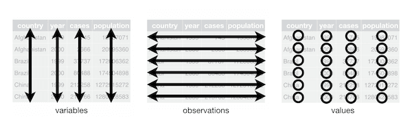
# ℹ 177 more rows

Reshaping with `pivot` functions

Converting into long or wide formats - pivot functions

The wide format is generally untidy but found in the majority of datasets and generally more readable.
The long format makes computation on columns sometimes easier.
- Use filter to compute on particular values.
The functions are called pivot_longer() and pivot_wider().

Pivot …

site	2001	2005	2015
L1002	120	100	105
L1034	125	130	140
L1234	100	110	105

longer

site	year	area
L1002	2001	120
L1002	2005	100
L1002	2015	105
L1034	2001	125
L1034	2005	130
L1034	2015	140
L1234	2001	100
L1234	2005	110
L1234	2015	105

Pivot …

site	year	area
L1002	2001	120
L1002	2005	100
L1002	2015	105
L1034	2001	125
L1034	2005	130
L1034	2015	140
L1234	2001	100
L1234	2005	110
L1234	2015	105

wider

site	2001	2005	2015
L1002	120	100	105
L1034	125	130	140
L1234	100	110	105

Making a wide data set longer

Calculations involving column and values

A toy data set

area_wide

# A tibble: 3 × 4
  site  `2001` `2005` `2015`
  <chr>  <dbl>  <dbl>  <dbl>
1 L1002    120    100    105
2 L1034    125    130    140
3 L1234    100    110    105

A longer table

area_long <- 
  pivot_longer(area_wide, 
  # columns to be transformed
  cols = !contains("site"), 
  names_to = "year",
   # We want to compute
  names_transform = as.numeric,
  values_to = "area")
area_long

# A tibble: 9 × 3
  site   year  area
  <chr> <dbl> <dbl>
1 L1002  2001   120
2 L1002  2005   100
3 L1002  2015   105
4 L1034  2001   125
5 L1034  2005   130
6 L1034  2015   140
7 L1234  2001   100
8 L1234  2005   110
9 L1234  2015   105

Making a wide data set longer

Calculations involving column and values

A toy data set

Variants by sample and positions.

variants_wide <- tribble(
  ~sample_id, ~`3`, ~`5`, ~`8`,
  "L1002",    "A",  "C",  NA,
  "L1034",    "A",  NA,   "T",
  "L1234",    NA,   "C",  "T"
)
variants_wide

# A tibble: 3 × 4
  sample_id `3`   `5`   `8`  
  <chr>     <chr> <chr> <chr>
1 L1002     A     C     <NA> 
2 L1034     A     <NA>  T    
3 L1234     <NA>  C     T

A longer, tidier table

variants_long <- 
  pivot_longer(variants_wide, 
  cols = -contains("sample"), # columns argument, required
  names_to = "pos",
  values_to = "variant")
variants_long

# A tibble: 9 × 3
  sample_id pos   variant
  <chr>     <chr> <chr>  
1 L1002     3     A      
2 L1002     5     C      
3 L1002     8     <NA>   
4 L1034     3     A      
5 L1034     5     <NA>   
6 L1034     8     T      
7 L1234     3     <NA>   
8 L1234     5     C      
9 L1234     8     T

Wider table

judgments |> 
  select(subject, condition, age, 
         starts_with("moral_dilemma") )

# A tibble: 188 × 10
   subject condition   age moral_dilemma_dog moral_dilemma_wallet moral_dilemma_plane moral_dilemma_resume
     <dbl> <chr>     <dbl>             <dbl>                <dbl>               <dbl>                <dbl>
 1       2 control      24                 9                    9                   8                    7
 2       1 stress       19                 9                    9                   9                    8
 3       3 stress       19                 8                    7                   8                    5
 4       4 stress       22                 8                    4                   8                    6
 5       7 control      22                 3                    9                   9                    5
 6       6 stress       22                 9                    9                   9                    9
 7       5 control      18                 9                    5                   7                    3
 8       9 control      20                 9                    4                   1                    7
 9      16 stress       21                 6                    9                   3                    9
10      13 stress       19                 6                    8                   9                    8
# ℹ 178 more rows
# ℹ 3 more variables: moral_dilemma_kitten <dbl>, moral_dilemma_trolley <dbl>, moral_dilemma_control <dbl>

Example

judgments |> 
  select(subject, condition, age, 
         starts_with("moral_dilemma") ) |> 
  pivot_longer(starts_with("moral_dilemma") , 
              names_to =  "dilemma",
              values_to = "dilemma_val",
              names_pattern = "moral_dilemma_(.*)")

# A tibble: 1,316 × 5
   subject condition   age dilemma dilemma_val
     <dbl> <chr>     <dbl> <chr>         <dbl>
 1       2 control      24 dog               9
 2       2 control      24 wallet            9
 3       2 control      24 plane             8
 4       2 control      24 resume            7
 5       2 control      24 kitten            9
 6       2 control      24 trolley           5
 7       2 control      24 control           9
 8       1 stress       19 dog               9
 9       1 stress       19 wallet            9
10       1 stress       19 plane             9
# ℹ 1,306 more rows

Example

judgments |> 
  select(subject, condition, age, 
         starts_with("moral_dilemma") ) |> 
  pivot_longer(starts_with("moral_dilemma") , 
              names_to =  "dilemma",
              values_to = "dilemma_val",
              names_pattern = "moral_dilemma_(.*)")  |> 
  count(condition, dilemma_val)

# A tibble: 18 × 3
   condition dilemma_val     n
   <chr>           <dbl> <int>
 1 control             1    25
 2 control             2    31
 3 control             3    48
 4 control             4    44
 5 control             5    49
 6 control             6    65
 7 control             7   103
 8 control             8   110
 9 control             9   162
10 stress              1    13
11 stress              2    35
12 stress              3    32
13 stress              4    51
14 stress              5    56
15 stress              6    54
16 stress              7   103
17 stress              8   133
18 stress              9   202

Example

judgments |> 
  select(subject, condition, age, 
         starts_with("moral_dilemma") ) |> 
  pivot_longer(starts_with("moral_dilemma") , 
              names_to =  "dilemma",
              values_to = "dilemma_val",
              names_pattern = "moral_dilemma_(.*)")  |> 
  count(condition, dilemma_val) |> 
  pivot_wider(names_from = dilemma_val, 
              values_from = n,
              names_prefix = "score")

# A tibble: 2 × 10
  condition score1 score2 score3 score4 score5 score6 score7 score8 score9
  <chr>      <int>  <int>  <int>  <int>  <int>  <int>  <int>  <int>  <int>
1 control       25     31     48     44     49     65    103    110    162
2 stress        13     35     32     51     56     54    103    133    202

Helpful tools

Removing the data frame context through `pull()`

Remark

By default tidyverse operations that receive a tibble as input return a tibble.

Extract column by name as vector

pull(judgments, age)[1:10]

 [1] 24 19 19 22 22 22 18 20 21 19

Extract same vector along with names

pull(judgments, age, name = subject)[1:10]

 2  1  3  4  7  6  5  9 16 13 
24 19 19 22 22 22 18 20 21 19

Comparing to data in other rows

Leading and lagging rows

lead() for data in following row and lag() for data in the row above

Calculate differences between subjects

Let’s assume the subject IDs are in order of the tests being conducted. What is the difference to the previous subject for the “initial mood”?

judgments |>
  select(subject, mood_pre) |> 
  arrange(subject) |> 
  mutate(prev_mood_pre = lag(mood_pre),
         mood_diff = mood_pre - lag(mood_pre))

# A tibble: 188 × 4
   subject mood_pre prev_mood_pre mood_diff
     <dbl>    <dbl>         <dbl>     <dbl>
 1       1       59            NA        NA
 2       2       81            59        22
 3       3       22            81       -59
 4       4       53            22        31
 5       5       NA            53        NA
 6       6       73            NA        NA
 7       7       48            73       -25
 8       8       59            48        11
 9       9      100            59        41
10      10       72           100       -28
# ℹ 178 more rows

The other 20% of `dplyr`

Occasionally handy

Assembly: bind_rows, bind_cols
Windows function, min_rank, dense_rank, cumsum. See vignette
Working with list-columns
multidplyr for parallelized code

SQL mapping allows database access

dplyr code can be translated into SQL and query databases online (using dbplyr)
Different types of tabular data (dplyr SQL backend, databases)

Your turn!

Exercises

Take the results from the previous exercise available as judgments_condition_stats and bring the data into a more readable format.

Make the table longer. After this step, your tibble should contain three columns:

The condition
the name of the moral dilemma and stats (in one column)
the values of the stats by moral dilemma.

Split the moral dilemma and stats column. You can use separate_wider_delim or mutate to create a column that contains the moral dilemma (dog, trolley, etc) and the stats (median, min, etc.).
Make the table wider again and move the stats to individual columns.

Your turn!

Exercises

The tribble contains changes of the sequence of a gene. The format in the input is the expected sequence (the reference allele), the position and the variant, commonly called alternative allele. In T6G, T is the reference allele, 6 is the position (along the gene) and G is the variant allele.

Clean the table of genetic variants such that all variants appear as a column labeled by their position.
Select relevant variants. In this table the variants are labeled according to their effect on stability of the gene product.
Identify the subjects in the table variants that carry variants labeled as damaging in variant_significance table. The final output should be vector of sample ids.

You can use several join flavours and the %in% operator to achieve the same result.

Input

```{r}
 tribble(
  ~sampleid, ~var1, ~var2, ~var3,
  "S1", "A3T", "T5G", "T6G",
  "S2", "A3G", "T5G", NA,
  "S3", "A3T", "T6C", "G10C",
  "S4", "A3T", "T6C", "G10C"
) 
```

15:00

Bigger data

Go for `data.table`

See this interesting thread about comparing data.table versus dplyr
data.table, see introduction is very efficient but the syntax is not so easy.
Main advantage: inline replacement (tidyverse is frequently copying)
As a summary: tl;dr data.table for speed, dplyr for readability and convenience Prashanth Sriram
Hadley recommends that for data > 1-2 Gb, if speed is your main matter, go for data.table
dtplyr is for learning the data.table from dplyr API input
tidytable is actually using data.table but with dplyr syntax
data.table might be not useful for specialized applications with high volumes such as genomics.

Before we stop

You learned to:

Joining and intersecting tibbles
Differ filtering from mutation joins
Reshaping column headers and variables

Further reading

R for Data Science:

Chapter 19 Joins

Acknowledgments

Hadley Wickham
Lionel Henry
Romain François
Lise Vaudor nice blog
Allison Horst for the great ArtWork
Alexandre Courtiol for cheatsheets
Jenny Bryan

Contributions

Milena Zizovic
Aurélien Ginolhac

Joins and pivots

Introduction

Motivation

Joining data frames

How do we refer to a particular observation?

Your turn!

Which columns are keys?

Solution

Primary key in judgments

Solution - Trees

Solution swiss

Mutating joins

Matching subjects in two tibbles

Additional data on coffee consumption

Smaller sample set

Combining the two tables

Inner join

Provide the corresponding columns names

Mutating joins

Inner join

Creating new tables through joins

Full Join

Example with full_join()

Two tables - same column names

Two tables - same column names

Join by one column

Join by two columns

Filtering joins

Filtering joins -

semi_join()

anti_join()

semi_join() to filter

Table x

Table y

Filtering

Mutating join

Inequality joins

Inequality joins

Redefine matches keys

Rewriting case_when()

Remember the tidyverse switch?

Rewriting case_when()

Remember the tidyverse switch?

Replacement

Replace with a table and a join

Join

Rolling join

Make it a rolling join with closest()

Replacement

Replace with a table and a join

Join

Rolling join

Make it a rolling join with closest()

Reshaping with pivot functions

Converting into long or wide formats - pivot functions

Pivot …

longer

Pivot …

wider

Making a wide data set longer

Calculations involving column and values

A toy data set

A longer table

Making a wide data set longer

Calculations involving column and values

A toy data set

A longer, tidier table

Wider table

Example

Example

Example

Helpful tools

Removing the data frame context through pull()

Remark

Extract column by name as vector

Extract same vector along with names

Comparing to data in other rows

Leading and lagging rows

Calculate differences between subjects

The other 20% of dplyr

Primary key in `judgments`

Solution `swiss`

Example with `full_join()`

`semi_join()`

`anti_join()`

`semi_join()` to filter

Rewriting `case_when()`

Remember the tidyverse `switch`?

Rewriting `case_when()`

Remember the tidyverse `switch`?

Make it a rolling join with `closest()`

Make it a rolling join with `closest()`

Reshaping with `pivot` functions

Removing the data frame context through `pull()`

The other 20% of `dplyr`

Go for `data.table`