Import Data

Loading with readr and readxl

Roland Krause

Rworkshop

Tuesday, 11 February 2025

Contents

• Importing text files
• Excel files

Introduction

Learning objectives

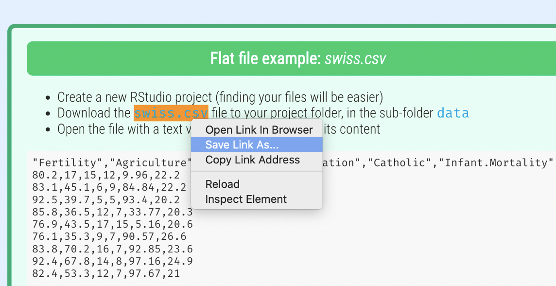
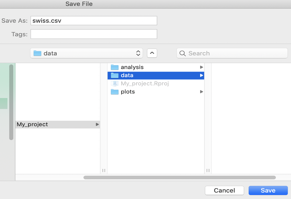
• Download a data file to a dedicated subfolder in your project
• Learn about tibbles
• Use readr to import flat-files data into R
• Use readxl to import excel files into R
• Hear tips about structuring your input

For now, no suggestion to use interactive downloading - more to show how to navigate in file browser

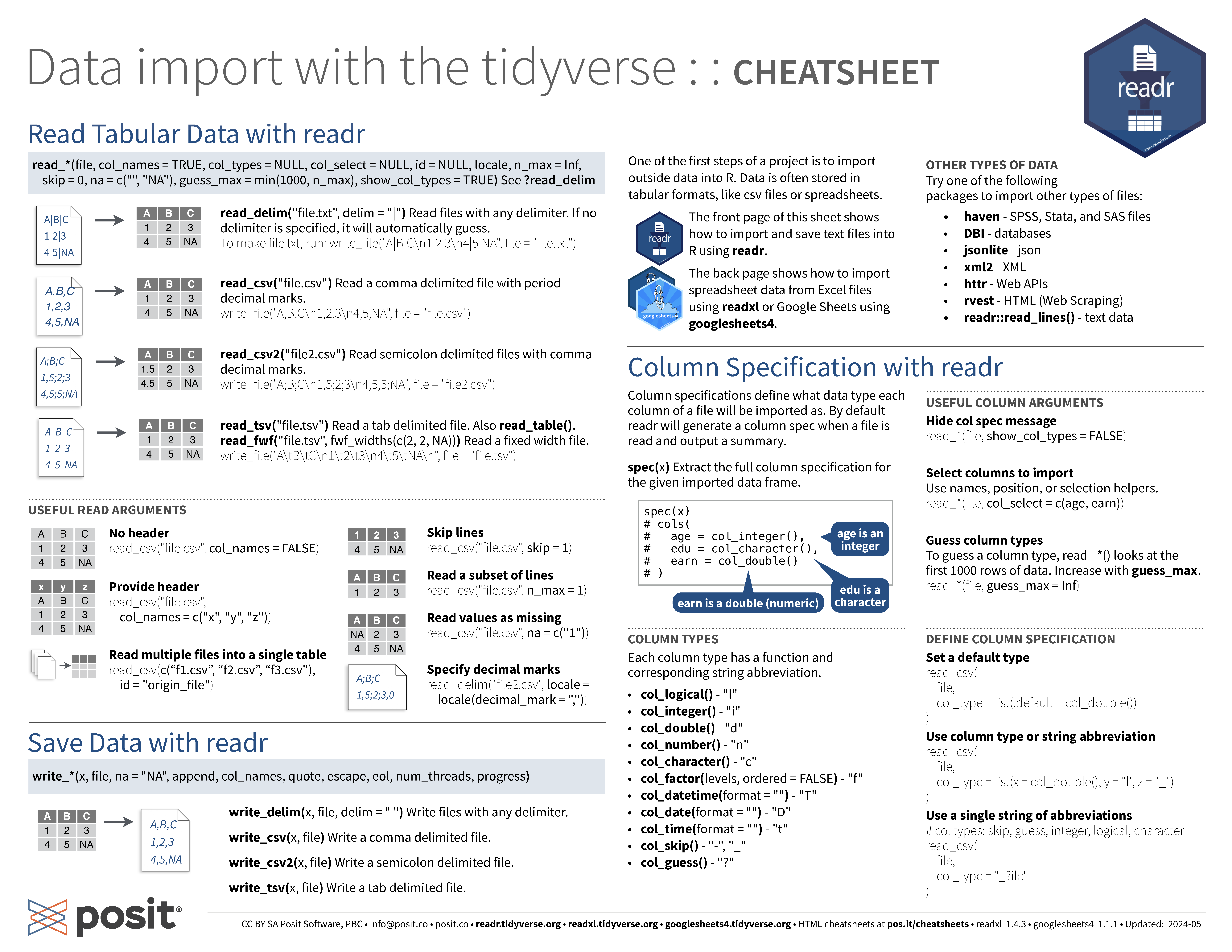
readr Cheatsheet

Importing data

The first step of your work

• But R base already provides functions for text files, e.g. read.csv()?

• What about …

  • Excel files (.xls, .xlsx)
  • Foreign statistical formats from SAS, SPSS or Stata
  • Databases (SQL, SQLite …)?

Tidyverse implementation

• More speed
• Improved handling of column types generates more consistent data structures
• Generates tibbles

Tibbles

• Have a refined print method that shows only the first 10 rows.
• Show all the columns that fit on screen and list the name of remaining ones.
• Each column reports its type (double, int, lgl, chr)
• Makes it much easier to work with long data tables

data.frame vs tibble

Data frame

swiss

             Fertility Agriculture Examination
Courtelary        80.2        17.0          15
Delemont          83.1        45.1           6
Franches-Mnt      92.5        39.7           5
Moutier           85.8        36.5          12
Neuveville        76.9        43.5          17
Porrentruy        76.1        35.3           9
Broye             83.8        70.2          16
Glane             92.4        67.8          14
Gruyere           82.4        53.3          12
Sarine            82.9        45.2          16
Veveyse           87.1        64.5          14
Aigle             64.1        62.0          21
Aubonne           66.9        67.5          14
Avenches          68.9        60.7          19
Cossonay          61.7        69.3          22
Echallens         68.3        72.6          18
Grandson          71.7        34.0          17
Lausanne          55.7        19.4          26
La Vallee         54.3        15.2          31
Lavaux            65.1        73.0          19
Morges            65.5        59.8          22
Moudon            65.0        55.1          14
Nyone             56.6        50.9          22
Orbe              57.4        54.1          20
Oron              72.5        71.2          12
Payerne           74.2        58.1          14
Paysd'enhaut      72.0        63.5           6
Rolle             60.5        60.8          16
Vevey             58.3        26.8          25
Yverdon           65.4        49.5          15
Conthey           75.5        85.9           3
Entremont         69.3        84.9           7
Herens            77.3        89.7           5
Martigwy          70.5        78.2          12
Monthey           79.4        64.9           7
St Maurice        65.0        75.9           9
Sierre            92.2        84.6           3
Sion              79.3        63.1          13
Boudry            70.4        38.4          26
La Chauxdfnd      65.7         7.7          29
Le Locle          72.7        16.7          22
Neuchatel         64.4        17.6          35
Val de Ruz        77.6        37.6          15
ValdeTravers      67.6        18.7          25
V. De Geneve      35.0         1.2          37
Rive Droite       44.7        46.6          16
Rive Gauche       42.8        27.7          22
             Education Catholic Infant.Mortality
Courtelary          12     9.96             22.2
Delemont             9    84.84             22.2
Franches-Mnt         5    93.40             20.2
Moutier              7    33.77             20.3
Neuveville          15     5.16             20.6
Porrentruy           7    90.57             26.6
Broye                7    92.85             23.6
Glane                8    97.16             24.9
Gruyere              7    97.67             21.0
Sarine              13    91.38             24.4
Veveyse              6    98.61             24.5
Aigle               12     8.52             16.5
Aubonne              7     2.27             19.1
Avenches            12     4.43             22.7
Cossonay             5     2.82             18.7
Echallens            2    24.20             21.2
Grandson             8     3.30             20.0
Lausanne            28    12.11             20.2
La Vallee           20     2.15             10.8
Lavaux               9     2.84             20.0
Morges              10     5.23             18.0
Moudon               3     4.52             22.4
Nyone               12    15.14             16.7
Orbe                 6     4.20             15.3
Oron                 1     2.40             21.0
Payerne              8     5.23             23.8
Paysd'enhaut         3     2.56             18.0
Rolle               10     7.72             16.3
Vevey               19    18.46             20.9
Yverdon              8     6.10             22.5
Conthey              2    99.71             15.1
Entremont            6    99.68             19.8
Herens               2   100.00             18.3
Martigwy             6    98.96             19.4
Monthey              3    98.22             20.2
St Maurice           9    99.06             17.8
Sierre               3    99.46             16.3
Sion                13    96.83             18.1
Boudry              12     5.62             20.3
La Chauxdfnd        11    13.79             20.5
Le Locle            13    11.22             18.9
Neuchatel           32    16.92             23.0
Val de Ruz           7     4.97             20.0
ValdeTravers         7     8.65             19.5
V. De Geneve        53    42.34             18.0
Rive Droite         29    50.43             18.2
Rive Gauche         29    58.33             19.3

Tibble

as_tibble(swiss)

# A tibble: 47 × 6
   Fertility Agriculture Examination Education
       <dbl>       <dbl>       <int>     <int>
 1      80.2        17            15        12
 2      83.1        45.1           6         9
 3      92.5        39.7           5         5
 4      85.8        36.5          12         7
 5      76.9        43.5          17        15
 6      76.1        35.3           9         7
 7      83.8        70.2          16         7
 8      92.4        67.8          14         8
 9      82.4        53.3          12         7
10      82.9        45.2          16        13
# ℹ 37 more rows
# ℹ 2 more variables: Catholic <dbl>,
#   Infant.Mortality <dbl>

Rownames in tibbles

Rownames

Base data frames have rownames, which a special type of column that need special treatments.

tibbles never use rownames!

When converting regular a data.frame they are lost unless you assign them to a dedicated column.

# library(tibble)
as_tibble(swiss, rownames = "Province")

# A tibble: 47 × 7
   Province     Fertility Agriculture Examination
   <chr>            <dbl>       <dbl>       <int>
 1 Courtelary        80.2        17            15
 2 Delemont          83.1        45.1           6
 3 Franches-Mnt      92.5        39.7           5
 4 Moutier           85.8        36.5          12
 5 Neuveville        76.9        43.5          17
 6 Porrentruy        76.1        35.3           9
 7 Broye             83.8        70.2          16
 8 Glane             92.4        67.8          14
 9 Gruyere           82.4        53.3          12
10 Sarine            82.9        45.2          16
# ℹ 37 more rows
# ℹ 3 more variables: Education <int>,
#   Catholic <dbl>, Infant.Mortality <dbl>

Importing data using readr function such as read_csv() will not create them.

Importing text files

Preparing the data

Description

Van ’t Veer, Anna; Sleegers, Willem. (2019) “Psychology data from an exploration of the effect of anticipatory stress on disgust vs. non-disgust related moral judgments”. Journal of Open Psychology Data.

• Moral dilemmata (trolley problem, survival after plane crash, etc. moral)
• Standard questionnaires
  • Private Body Consciousness (PBC, range 0 - 4)
  • Rational-Experiential Inventory (REI, range 1 - 5)
  • Multidimensional Assessment of Interoceptive Awareness (MAIA, range 0 - 5 )
  • State Trait Anxiety Inventory (STAI)

judge_url <- "https://biostat2.uni.lu/practicals/data/judgments.tsv"
judgments <- readr::read_tsv(judge_url)
# https://dataverse.nl/api/access/datafile/11863
#"https://biostat2.uni.lu/practicals/data/judgments.tsv")

Your turn!

Load the data into your RStudio session if you wish to follow along

02:00

judgments <- readr::read_tsv("data/judgments.tsv", show_col_types = FALSE)
judgments

# A tibble: 188 × 158
   start_date end_date  finished condition subject
   <chr>      <chr>        <dbl> <chr>       <dbl>
 1 11/3/2014  11/3/2014        1 control         2
 2 11/3/2014  11/3/2014        1 stress          1
 3 11/3/2014  11/3/2014        1 stress          3
 4 11/3/2014  11/3/2014        1 stress          4
 5 11/3/2014  11/3/2014        1 control         7
 6 11/3/2014  11/3/2014        1 stress          6
 7 11/3/2014  11/3/2014        1 control         5
 8 11/3/2014  11/3/2014        1 control         9
 9 11/3/2014  11/3/2014        1 stress         16
10 11/3/2014  11/3/2014        1 stress         13
# ℹ 178 more rows
# ℹ 153 more variables: gender <chr>, age <dbl>,
#   mood_pre <dbl>, mood_post <dbl>,
#   STAI_pre_1_1 <dbl>, STAI_pre_1_2 <dbl>,
#   STAI_pre_1_3 <dbl>, STAI_pre_1_4 <dbl>,
#   STAI_pre_1_5 <dbl>, STAI_pre_1_6 <dbl>,
#   STAI_pre_1_7 <dbl>, STAI_pre_2_1 <dbl>, …

Your turn

Downloading files

• Download the judgments.tsv file to your project directory data

download.file("https://biostat2.uni.lu/practicals/data/judgments.tsv",
"data/judgments.tsv")

• Open the file with a text viewer and have a look at its content!
• Does the delimiter fit the file extension?
• Read the file into the session with read_delim() and assign the name judgments.

judgments <- readr::read_delim("data/judgments.tsv")

Use the RStudio project!

Finding your files will be easier.

Inspection

Did we load the data correctly?

Check with

spec(judgments)

cols(
  start_date = col_character(),
  end_date = col_character(),
  finished = col_double(),
  condition = col_character(),
  subject = col_double(),
  gender = col_character(),
  age = col_double(),
  mood_pre = col_double(),
  mood_post = col_double(),
  STAI_pre_1_1 = col_double(),
  STAI_pre_1_2 = col_double(),
  STAI_pre_1_3 = col_double(),
  STAI_pre_1_4 = col_double(),
  STAI_pre_1_5 = col_double(),
  STAI_pre_1_6 = col_double(),
  STAI_pre_1_7 = col_double(),
  STAI_pre_2_1 = col_double(),
  STAI_pre_2_2 = col_double(),
  STAI_pre_2_3 = col_double(),
  STAI_pre_2_4 = col_double(),
  STAI_pre_2_5 = col_double(),
  STAI_pre_2_6 = col_double(),
  STAI_pre_2_7 = col_double(),
  STAI_pre_3_1 = col_double(),
  STAI_pre_3_2 = col_double(),
  STAI_pre_3_3 = col_double(),
  STAI_pre_3_4 = col_double(),
  STAI_pre_3_5 = col_double(),
  STAI_pre_3_6 = col_double(),
  STAI_post_1_1 = col_double(),
  STAI_post_1_2 = col_double(),
  STAI_post_1_3 = col_double(),
  STAI_post_1_4 = col_double(),
  STAI_post_1_5 = col_double(),
  STAI_post_1_6 = col_double(),
  STAI_post_1_7 = col_double(),
  STAI_post_2_1 = col_double(),
  STAI_post_2_2 = col_double(),
  STAI_post_2_3 = col_double(),
  STAI_post_2_4 = col_double(),
  STAI_post_2_5 = col_double(),
  STAI_post_2_6 = col_double(),
  STAI_post_2_7 = col_double(),
  STAI_post_3_1 = col_double(),
  STAI_post_3_2 = col_double(),
  STAI_post_3_3 = col_double(),
  STAI_post_3_4 = col_double(),
  STAI_post_3_5 = col_double(),
  STAI_post_3_6 = col_double(),
  moral_dilemma_dog = col_double(),
  moral_dilemma_wallet = col_double(),
  moral_dilemma_plane = col_double(),
  moral_dilemma_resume = col_double(),
  moral_dilemma_kitten = col_double(),
  moral_dilemma_trolley = col_double(),
  moral_dilemma_control = col_double(),
  presentation_experience = col_double(),
  presentation_unpleasant = col_double(),
  presentation_fun = col_double(),
  presentation_challenge = col_double(),
  PBC_1 = col_double(),
  PBC_2 = col_double(),
  PBC_3 = col_double(),
  PBC_4 = col_double(),
  PBC_5 = col_double(),
  REI_1 = col_double(),
  REI_2 = col_double(),
  REI_3 = col_double(),
  REI_4 = col_double(),
  REI_5 = col_double(),
  REI_6 = col_double(),
  REI_7 = col_double(),
  REI_8 = col_double(),
  REI_9 = col_double(),
  REI_10 = col_double(),
  REI_11 = col_double(),
  REI_12 = col_double(),
  REI_13 = col_double(),
  REI_14 = col_double(),
  REI_15 = col_double(),
  REI_16 = col_double(),
  REI_17 = col_double(),
  REI_18 = col_double(),
  REI_19 = col_double(),
  REI_20 = col_double(),
  REI_21 = col_double(),
  REI_22 = col_double(),
  REI_23 = col_double(),
  REI_24 = col_double(),
  REI_25 = col_double(),
  REI_26 = col_double(),
  REI_27 = col_double(),
  REI_28 = col_double(),
  REI_29 = col_double(),
  REI_30 = col_double(),
  REI_31 = col_double(),
  REI_32 = col_double(),
  REI_33 = col_double(),
  REI_34 = col_double(),
  REI_35 = col_double(),
  REI_36 = col_double(),
  REI_37 = col_double(),
  REI_38 = col_double(),
  REI_39 = col_double(),
  REI_40 = col_double(),
  MAIA_1_1 = col_double(),
  MAIA_1_2 = col_double(),
  MAIA_1_3 = col_double(),
  MAIA_1_4 = col_double(),
  MAIA_1_5 = col_double(),
  MAIA_1_6 = col_double(),
  MAIA_1_7 = col_double(),
  MAIA_1_8 = col_double(),
  MAIA_1_9 = col_double(),
  MAIA_1_10 = col_double(),
  MAIA_1_11 = col_double(),
  MAIA_1_12 = col_double(),
  MAIA_1_13 = col_double(),
  MAIA_1_14 = col_double(),
  MAIA_1_15 = col_double(),
  MAIA_1_16 = col_double(),
  MAIA_2_1 = col_double(),
  MAIA_2_2 = col_double(),
  MAIA_2_3 = col_double(),
  MAIA_2_4 = col_double(),
  MAIA_2_5 = col_double(),
  MAIA_2_6 = col_double(),
  MAIA_2_7 = col_double(),
  MAIA_2_8 = col_double(),
  MAIA_2_9 = col_double(),
  MAIA_2_10 = col_double(),
  MAIA_2_11 = col_double(),
  MAIA_2_12 = col_double(),
  MAIA_2_13 = col_double(),
  MAIA_2_14 = col_double(),
  MAIA_2_15 = col_double(),
  MAIA_2_16 = col_double(),
  STAI_pre = col_double(),
  STAI_post = col_double(),
  MAIA_noticing = col_double(),
  MAIA_not_distracting = col_double(),
  MAIA_not_worrying = col_double(),
  MAIA_attention_regulation = col_double(),
  MAIA_emotional_awareness = col_double(),
  MAIA_self_regulation = col_double(),
  MAIA_body_listening = col_double(),
  MAIA_trusting = col_double(),
  PBC = col_double(),
  REI_rational_ability = col_double(),
  REI_rational_engagement = col_double(),
  REI_experiental_ability = col_double(),
  REI_experiental_engagement = col_double(),
  moral_judgment = col_double(),
  moral_judgment_disgust = col_double(),
  moral_judgment_non_disgust = col_double(),
  presentation_evaluation = col_double(),
  logbook = col_character(),
  exclude = col_double()
)

Do all columns have the correct data type?

Answers expected or hinted at from audience - numbers are integers - dates should be in data formats - some characters should be factors, not text

Manual download

In your browser:

• Right-click on the link
• Choose Save Link As

• Use Finder/Explorer to select this project folder
• Go inside this sub-folder data
• Hit Save

Data types and classes in R

Data types

Type	Example
numeric	integer (2), double (2.34)
character (strings)	"tidyverse!"
boolean	TRUE / FALSE (T/F not protected)
complex	2+0i

Data classes

Class	Example
Factors	factor(c("a", "b"))
Date	as.Date("2025-02-10")
Datetime	as.POSIXct("2025-01-03 14:00")
Time (difftime)	Result of computation of Datetime

Missing data

Class	Description
NA	not available, missing data
NA_real_	Double type
NA_integer_	Integer type
NA_character_	Character type
NA_complex_	Complex type
NULL	Vector of lenght zero
-Inf/Inf	Infinite values
NaN	Not a Number

Treat missing data as missing

One can

• remove observation,
• impute a suitable values,
• set to neutral category.

Context-dependent and can be very relevant to your analyses.

Include missing data as category in your exploratory analysis.

Column types

Function	Short	Description
col_logical()	l	TRUE/FALSE, 1/0
col_integer()	i	Integers
col_double()	d	Floating point values.
col_number()	n	Numbers removing non-number elements
col_date(format = "")	D	<date>
col_time(format = "")	t	<dttm>
col_datetime(format = "")	T	<datetime>
col_factor(levels, ordered)	f	Categorical or ordinal data
col_character()	c	Everything else
col_skip()	_	Do not import this column
col_guess()	?	Parse using the “best” type based on the input

All columns are selected with cols()

Column types can be specified using col_types = cols()

Separate argument col_select for restricting column selection.

Column selection with tidyselect

Lighter column type definitions

Use tidyselect helpers

readr::read_delim("data/judgments.tsv",
                  col_select = c(subject,
                                 starts_with("STAI")))

# A tibble: 188 × 43
   subject STAI_pre_1_1 STAI_pre_1_2 STAI_pre_1_3
     <dbl>        <dbl>        <dbl>        <dbl>
 1       2            2            1            2
 2       1            3            2            3
 3       3            4            3            3
 4       4            2            2            2
 5       7            1            1            1
 6       6            2            2            1
 7       5            2            2            1
 8       9            1            1            1
 9      16            2            2            1
10      13            4            2            3
# ℹ 178 more rows
# ℹ 39 more variables: STAI_pre_1_4 <dbl>,
#   STAI_pre_1_5 <dbl>, STAI_pre_1_6 <dbl>,
#   STAI_pre_1_7 <dbl>, STAI_pre_2_1 <dbl>,
#   STAI_pre_2_2 <dbl>, STAI_pre_2_3 <dbl>,
#   STAI_pre_2_4 <dbl>, STAI_pre_2_5 <dbl>,
#   STAI_pre_2_6 <dbl>, STAI_pre_2_7 <dbl>, …

Tip

This package is the backend for programatic column selection in the tidyverse. Features are described in this article.

Operators and helper functions

Expression	Description
[c()]	Combining bare names
[:]	Selecting a range
[!]	Negating a selection
everything()	All columns
last_col()	Last column
starts_with()	Quoted prefix
ends_with()	Quoted suffix
contains()	Quoted string
matches()	Regular expression

Catch and report reading issues

Specifying column types with cols()

readr records issues. Use problems() to see them

jud2 <- readr::read_delim("data/judgments.tsv",
             col_types = cols(start_date = col_date(),
                              end_date = col_date()))

jud2

# A tibble: 188 × 158
   start_date end_date finished condition
   <date>     <date>      <dbl> <chr>    
 1 NA         NA              1 control  
 2 NA         NA              1 stress   
 3 NA         NA              1 stress   
 4 NA         NA              1 stress   
 5 NA         NA              1 control  
 6 NA         NA              1 stress   
 7 NA         NA              1 control  
 8 NA         NA              1 control  
 9 NA         NA              1 stress   
10 NA         NA              1 stress   
# ℹ 178 more rows
# ℹ 154 more variables: subject <dbl>,
#   gender <chr>, age <dbl>, mood_pre <dbl>,
#   mood_post <dbl>, STAI_pre_1_1 <dbl>,
#   STAI_pre_1_2 <dbl>, STAI_pre_1_3 <dbl>,
#   STAI_pre_1_4 <dbl>, STAI_pre_1_5 <dbl>,
#   STAI_pre_1_6 <dbl>, STAI_pre_1_7 <dbl>, …

problems(jud2)

# A tibble: 376 × 5
     row   col expected        actual    file     
   <int> <int> <chr>           <chr>     <chr>    
 1     2     1 date in ISO8601 11/3/2014 /builds/…
 2     2     2 date in ISO8601 11/3/2014 /builds/…
 3     3     1 date in ISO8601 11/3/2014 /builds/…
 4     3     2 date in ISO8601 11/3/2014 /builds/…
 5     4     1 date in ISO8601 11/3/2014 /builds/…
 6     4     2 date in ISO8601 11/3/2014 /builds/…
 7     5     1 date in ISO8601 11/3/2014 /builds/…
 8     5     2 date in ISO8601 11/3/2014 /builds/…
 9     6     1 date in ISO8601 11/3/2014 /builds/…
10     6     2 date in ISO8601 11/3/2014 /builds/…
# ℹ 366 more rows

Correct data input

jud2 <- readr::read_delim("data/judgments.tsv",
             col_types = 
               cols(start_date = col_date(format = "%d/%m/%Y"),
                    end_date = col_date(format =  "%d/%m/%Y"),
                    finished = "f",
                    condition = "f",
                    gender = "f",
                    logbook = "c", 
                    exclude = "f",
                    moral_judgment = "d",
                    moral_judgment_disgust = "d",
                    moral_judgment_non_disgust = "d",
                    .default = col_integer()))

jud2

# A tibble: 188 × 158
   start_date end_date   finished condition
   <date>     <date>     <fct>    <fct>    
 1 2014-03-11 2014-03-11 1        control  
 2 2014-03-11 2014-03-11 1        stress   
 3 2014-03-11 2014-03-11 1        stress   
 4 2014-03-11 2014-03-11 1        stress   
 5 2014-03-11 2014-03-11 1        control  
 6 2014-03-11 2014-03-11 1        stress   
 7 2014-03-11 2014-03-11 1        control  
 8 2014-03-11 2014-03-11 1        control  
 9 2014-03-11 2014-03-11 1        stress   
10 2014-03-11 2014-03-11 1        stress   
# ℹ 178 more rows
# ℹ 154 more variables: subject <int>,
#   gender <fct>, age <int>, mood_pre <int>,
#   mood_post <int>, STAI_pre_1_1 <int>,
#   STAI_pre_1_2 <int>, STAI_pre_1_3 <int>,
#   STAI_pre_1_4 <int>, STAI_pre_1_5 <int>,
#   STAI_pre_1_6 <int>, STAI_pre_1_7 <int>, …

Reading data with no column header

Example

The animal data contains three columns and three rows.

dog,red,1
cat,blue,2
chicken,green,6

Naive approach

animal_file <- "data/animals.csv"
readr::read_delim(animal_file)

# A tibble: 2 × 3
  dog     red     `1`
  <chr>   <chr> <dbl>
1 cat     blue      2
2 chicken green     6

Satisfying?

Read all lines

read_delim(animal_file, col_names = FALSE, show_col_types = FALSE)

# A tibble: 3 × 3
  X1      X2       X3
  <chr>   <chr> <dbl>
1 dog     red       1
2 cat     blue      2
3 chicken green     6

Satisfying?

• Colnames are self-created.
• show_col_types = FALSE suppresses the verbose mode

Supply the colnames

read_delim(animal_file, 
           col_names = c("animal", "color", "value"),
           show_col_types = FALSE)

# A tibble: 3 × 3
  animal  color value
  <chr>   <chr> <dbl>
1 dog     red       1
2 cat     blue      2
3 chicken green     6

Better

Examples for data-aware inputs

Using one-letter shortcuts

readr::read_delim(animal_file, 
      col_names = c("animal", "color", "value"),
      col_types = cols(
        animal = "c",
        color = "_",
        value = "i"
      ))

# A tibble: 3 × 2
  animal  value
  <chr>   <int>
1 dog         1
2 cat         2
3 chicken     6

Even more compact

readr::read_delim(animal_file, 
      col_names = c("animal", "color", "value"),
      col_types = "c_i")

# A tibble: 3 × 2
  animal  value
  <chr>   <int>
1 dog         1
2 cat         2
3 chicken     6

• Use the single character code in the column order

Skipping lines

Our example

# A tibble: 3 × 2
  animal  value
  <chr>   <int>
1 dog         1
2 cat         2
3 chicken     6

Comment

readr::read_delim(
  animal_file,
  comment = "d",
  col_names = FALSE,
  show_col_types = FALSE)

# A tibble: 2 × 3
  X1      X2       X3
  <chr>   <chr> <dbl>
1 cat     blue      2
2 chicken green     6

Do not read lines beginning with a character.

Skip lines

readr::read_delim(
  animal_file,
  skip = 1, 
  col_names = FALSE,
  show_col_types = FALSE)

# A tibble: 2 × 3
  X1      X2       X3
  <chr>   <chr> <dbl>
1 cat     blue      2
2 chicken green     6

Limited number of lines

readr::read_delim(
  animal_file,
  skip = 1,
  n_max = 1,
  col_names = FALSE,
  show_col_types = FALSE
)

# A tibble: 1 × 3
  X1    X2       X3
  <chr> <chr> <dbl>
1 cat   blue      2

Several files at once

Multiple files are read into one tibble

readr::read_csv(c("data/swiss.csv",  "data/swiss.csv"))

# A tibble: 94 × 6
   Fertility Agriculture Examination Education
       <dbl>       <dbl>       <dbl>     <dbl>
 1      80.2        17            15        12
 2      83.1        45.1           6         9
 3      92.5        39.7           5         5
 4      85.8        36.5          12         7
 5      76.9        43.5          17        15
 6      76.1        35.3           9         7
 7      83.8        70.2          16         7
 8      92.4        67.8          14         8
 9      82.4        53.3          12         7
10      82.9        45.2          16        13
# ℹ 84 more rows
# ℹ 2 more variables: Catholic <dbl>,
#   Infant.Mortality <dbl>

Files with different columns are not read

readr::read_csv(c("data/swiss.csv", "data/swiss2.csv"))

Error: Files must all have 6 columns:
* File 2 has 5 columns

Filenames as extra column

File names are recorded by providing the id argument.

options(width = 100)
readr::read_csv(c("data/swiss_ray.csv", "data/swiss.csv"),
                 col_name = c("fer", "agri", "exa", "edu",
                              "cath", "inf", "ray"),
                id =  "orig",
                show_col_types = FALSE)

# A tibble: 54 × 7
   orig               fer       agri        exa         edu       cath     inf             
   <chr>              <chr>     <chr>       <chr>       <chr>     <chr>    <chr>           
 1 data/swiss_ray.csv fer       agri        exa         edu       cath     xray            
 2 data/swiss_ray.csv 80.2      17          15          12        <NA>     <NA>            
 3 data/swiss_ray.csv a         45.1        6           9         84.8     <NA>            
 4 data/swiss_ray.csv 92.5      39.7        5           5         <NA>     <NA>            
 5 data/swiss_ray.csv 85.8      36.5        12          7         33.8     <NA>            
 6 data/swiss_ray.csv 76.9      43.5        17          15        5.16     <NA>            
 7 data/swiss.csv     Fertility Agriculture Examination Education Catholic Infant.Mortality
 8 data/swiss.csv     80.2      17          15          12        9.96     22.2            
 9 data/swiss.csv     83.1      45.1        6           9         84.84    22.2            
10 data/swiss.csv     92.5      39.7        5           5         93.4     20.2            
# ℹ 44 more rows

Can you spot the error?

Pass the input column names if not in agreement.

Reading in multiple files of different formats

Reading in many files, e.g. database tables can be cumbersome.

Read into a list or data.frame structure (see nesting in tidyr)

• Rectangling vignette

Tricks and tips

Loading zipped files from the web

Loading from the web

read_csv("https://biostat2.uni.lu/practicals/data/swiss.csv")

# A tibble: 47 × 6
   Fertility Agriculture Examination Education
       <dbl>       <dbl>       <dbl>     <dbl>
 1      80.2        17            15        12
 2      83.1        45.1           6         9
 3      92.5        39.7           5         5
 4      85.8        36.5          12         7
 5      76.9        43.5          17        15
 6      76.1        35.3           9         7
 7      83.8        70.2          16         7
 8      92.4        67.8          14         8
 9      82.4        53.3          12         7
10      82.9        45.2          16        13
# ℹ 37 more rows
# ℹ 2 more variables: Catholic <dbl>,
#   Infant.Mortality <dbl>

No need to download files.

Reading zipped files

read_csv("data/mtcars.csv.gz")

# A tibble: 32 × 11
     mpg   cyl  disp    hp  drat    wt  qsec    vs
   <dbl> <dbl> <dbl> <dbl> <dbl> <dbl> <dbl> <dbl>
 1  21       6  160    110  3.9   2.62  16.5     0
 2  21       6  160    110  3.9   2.88  17.0     0
 3  22.8     4  108     93  3.85  2.32  18.6     1
 4  21.4     6  258    110  3.08  3.22  19.4     1
 5  18.7     8  360    175  3.15  3.44  17.0     0
 6  18.1     6  225    105  2.76  3.46  20.2     1
 7  14.3     8  360    245  3.21  3.57  15.8     0
 8  24.4     4  147.    62  3.69  3.19  20       1
 9  22.8     4  141.    95  3.92  3.15  22.9     1
10  19.2     6  168.   123  3.92  3.44  18.3     1
# ℹ 22 more rows
# ℹ 3 more variables: am <dbl>, gear <dbl>,
#   carb <dbl>

Excel files

Reading Excel files

readxl package is part of tidyverse and makes it easy to import tabular data from Excel spreadsheets with several options.

More details are described in this pkgdown website

Features

• readxl author: Hadley Wickham and Jenny Bryan
• read_excel() reads both xls and xlsx files and detects the format from the extension. Otherwise:
  • read_xls()
  • read_xlsx()
• Return tibbles
• Column type guessing
• Discovers the minimal data rectangle and returns that, by default
• No external library dependencies, e.g., Java or Perl

Usage guidance

• Exert more control with range, skip, and n_max
• excel_sheets() returns the sheet names
• Combine multiple sheets, jointly with purrr::map_df()
• col_types arguments match Excel’s data types
  • “numeric”, “text”, “skip”, “guess”,

The tidyverse packages to import your data

readr

• read_csv(): comma separated (,)
• read_csv2(): separated (;)
• read_tsv(): tab separated
• read_delim(): general delimited files, auto-guesses delimiter
• read_fwf(): fixed width files
• read_table(): columns separated by white-space(s)

readxl

• read_excel()
• read_xls()
• read_xlsx()

haven

• read_sas() for SAS
• read_sav() for SPSS
• read_dta() for Stata

Additions to readr and readxl

Need for (more) speed

Check fread() from data.table

• Stable, no dependencies
• Could feed from bash command
• Could be faster than readr functions
• Only relevant if you have data sets in the Gbyte range to read

Import Google spreadsheets

• Google spreadsheet can be read with googlesheets4 package
• Well developed package

Import Excel cell color

Check the tidyxl package to expose all content, cell by cell.

Good to know

Hell are other people’s column names

Fixing column names on import

Duplicated, Missing, Ugly (e.g. - , %)

Colnames are repaired with several options for their treatment ("minimal", "unique", "universal", "check_unique").

See details in the vctrs package description.

readxl::read_excel(
  "data/bad-table-psych.xlsx",
  skip = 2,
  n_max = 12,
  .name_repair = "universal"
) |>
  rename_with(\(x) str_to_lower(x))  |>
  rename_with(\(x) str_replace_all(x, "\\.+", "_"))

# A tibble: 12 × 18
   name        id gender language_4 birthday `_6` 
   <chr>    <dbl> <chr>  <chr>      <chr>    <lgl>
 1 Roland …     1 male   German     38687    NA   
 2 Lars Ju…     2 m      German     26/2/19… NA   
 3 <NA>         2 m      GErman     26/2/19… NA   
 4 <NA>         2 male   German     26/2/19… NA   
 5 Martina…     4 f      German     12-03-2… NA   
 6 Horst-S…     5 m      French     12/11/70 NA   
 7 Horst-S…     5 <NA>   <NA>       11-12-70 NA   
 8 LJK          7 f      Französis… <NA>     NA   
 9 DFK          8 f      Französis… 2005-12… NA   
10 Horst M…     9 male   Deutsch    1972-10… NA   
11 Kevin M…    10 männl… Deutsch    5.4.1970 NA   
12 Inga Mo…    11 weibl… Deutsch    1/1/1990 NA   
# ℹ 12 more variables: test_reaction <chr>,
#   morale_by_stai_test_ <lgl>, `_9` <dbl>,
#   stai <chr>, language_11 <chr>, `_12` <lgl>,
#   rec_1 <dbl>, rec_2 <dbl>, rec_3 <dbl>,
#   language_16 <chr>, `_17` <lgl>, comment <chr>

Best practices

General advice

• Structure your input data process.
• Load all data early in your process and in a central place unless there are specific performance issues.
• Re-factor your inputs, don’t rely on changing things during analysis.
• Do not read the whole file just because you can for your production code.
• Avoid downloading manually - use API calls or download data programmatically for external data unless size or availability becomes an issue.

Tidy imports

• Check the cheat sheet
• Read columns you want explicitly with appropriate col_types()
• You tidyselect helpers to specify many similar columns
• Clean up column names with dplyr and stringr functions early.

Before we stop

You learned to:

• Appreciate the tibble features
• Learn set-up working directory with RStudio projects
• Learn the tidyselect syntax
• Use readr::read_delim to import your flat files
• Adjust the imported data types
• Use readxl to import excel files

Further reading

Check R for Data Science for Import and Spreadsheets.

Contains information on databases and specialised formats.

Acknowledgments

• Development:

• Eric Koncina (initial installment)

• Veronica Codoni (swiss data set)

• Aurélien Ginolhac (vroom development)

• Roland Krause (readr 2.0 update)

• Input and inspiration:

• Jim Hester (vroom, readr development)

• Jenny Bryan (advice with project organization)

• Hadley Wickham

• Nicholas Tierney

Thank you for your attention!