Advanced R
for Functional Programming
Roland Krause
R Workshop
Wednesday, 12 February 2025
Introduction
Material
- purrr Tutorial by Jenny Bryan
R for Data Science
Advanced R
- Functions
- Functional programming
- Several chapters
Learning objectives
Learning objectives
Functional programming approach to focus on
actionsIteration machinery written by someone else
Pass
functionsasargumentsto higher order functionsUse
map()to replace remainingforloopsWorking with lists
Nesting of data
Outlook
Building multiple models from tidy data (
purrr)Working with multiple models (
broom, next lecture)
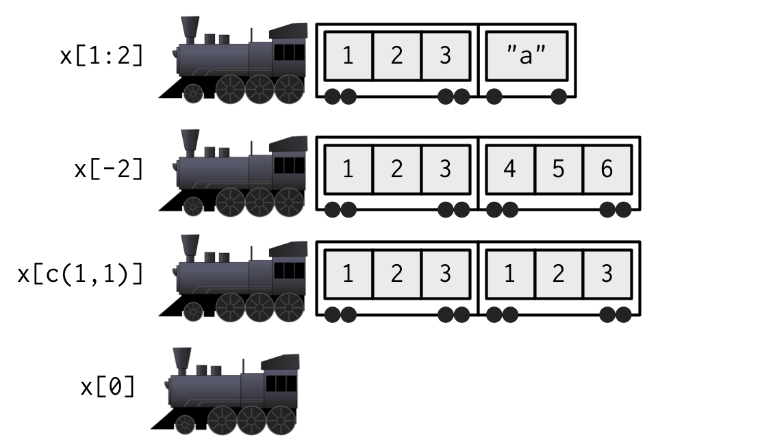
Types and classes
Types and classes
Retrieve the data type with typeof()
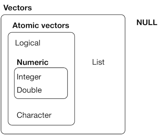
Vectors
Atomic vectors
Atomic means only one type of data
The type of each atom is the same. The size of each atom is one single element.
The conversion between types can be
- Explicit (using
as.*()functions) - or Implicit
Factors
Categorical values
Factors are useful - to restrict possible values - to order character values
Using strings
Rivers flow into each other but sort() would not know.
Unordered by default
Creating an ordered list
(rivers_fct <- factor(rivers_str,
                      levels = c("Alzette", "Sauer", "Moselle", "Rhine"),
                        ordered = TRUE))
[1] Alzette Moselle Rhine Sauer
Levels: Alzette < Sauer < Moselle < Rhineforcats
Factors are seen in statistical applications and plotting order. Manipulation of factors is greatly simplified by the forcats package.
We will exercise this in the context of ggplot.
Date and Time are inbuilt classes
Converting to dates
This year as Date
Import
# A tibble: 1 × 1
  year
  <date>
1 2024-01-01
lubridate to the rescue
lubridate cheatsheet
You can do a lot of things in base R with dates without lubridate but it provides an excellent cheatsheet lubridate has a range of functions for parsing ill-formatted dates and times.
Parsing dates with lubridate functions (reprise)
A gift from your collaborators
Lubridate to the rescue!
# A tibble: 5 × 3
  subject visit_date   good_date
    <dbl> <chr>        <date>
1       1 01/07/2001   2001-07-01
2       2 01.MAY.2012  2012-05-01
3       3 12-07-2015   2015-07-12
4       4 4/5/14       2014-05-04
5       5 12. Jun 1999 1999-06-12
All dates must use date types
Don’t be cheap - it’s easy to convert dates to date; all major programming environments support date and time classes.
Your turn!
Find three ways of expressing the names of the twelve months that will sort correctly.
15:00
Lists
Introduction to lists
source: H. Wickham - R for data science, licence CC
Lists are cool
Can contain anything, named or not
[[1]]
  height weight
1     58    115
2     59    117
3     60    120

$sw
             Fertility Agriculture Examination Education Catholic
Courtelary        80.2        17.0          15        12     9.96
Delemont          83.1        45.1           6         9    84.84
Franches-Mnt      92.5        39.7           5         5    93.40
             Infant.Mortality
Courtelary               22.2
Delemont                 22.2
Franches-Mnt             20.2

[[3]]
[1] "ab" "c"
Even empty slot
[[1]]
  height weight
1     58    115
2     59    117
3     60    120

[[2]]
NULL

$sw
             Fertility Agriculture Examination Education Catholic
Courtelary        80.2        17.0          15        12     9.96
Delemont          83.1        45.1           6         9    84.84
Franches-Mnt      92.5        39.7           5         5    93.40
             Infant.Mortality
Courtelary               22.2
Delemont                 22.2
Franches-Mnt             20.2

[[4]]
[1] "ab" "c"
Working with lists
Accessing elements of a list
The steam machine is the list() structure 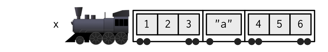
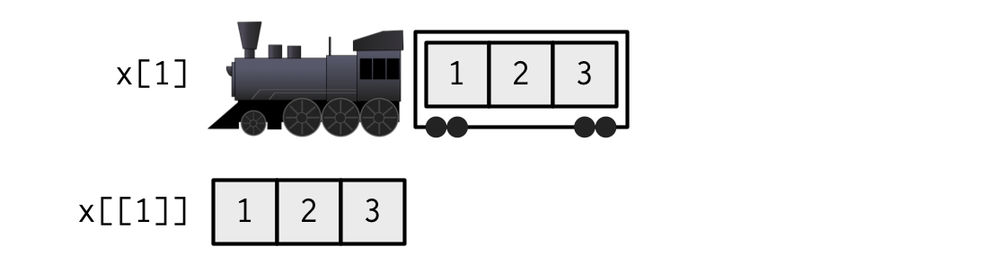
[["element]] == $element
The $ notation is a shorthand for the double brackets that does not require quoting the name of the item.
Sub-selection
from Advanced R, second Ed. by Hadley Wickham
Lists inside rectangle data
Rectangle, tibble/data.frame fits our mindset
2D representation of data we see everywhere
# A tibble: 4 × 5
  ccn    facility_name    measure_abbr score type
  <chr>  <chr>            <chr>        <dbl> <chr>
1 011502 COMFORT CARE CO… visits_immi…   390 deno…
2 011517 HOSPICE OF WEST… pain_assess…   100 obse…
3 011508 SOUTHERNCARE NE… opioid_bowel   100 obse…
4 011501 SOUTHERNCARE NE… pain_assess… 325 deno…- Are columns with more complex structures useful?
- Can we not model everything flat?
- How to store some JSON?
Use list-columns
cms |>
  mutate(metadata = list(
    women,
    vec = c("ab", "c"),
    lm(height ~ weight, data = women),
    NULL
  ), .after = ccn)
# A tibble: 4 × 6
ccn metadata facility_name measure_abbr score
<chr> <named > <chr> <chr> <dbl>
1 011502 <df> COMFORT CARE… visits_immi… 390
2 011517 <chr> HOSPICE OF W… pain_assess… 100
3 011508 <lm> SOUTHERNCARE… opioid_bowel 100
4 011501 <NULL> SOUTHERNCARE… pain_assess… 325
# ℹ 1 more variable: type <chr>- However, how can we iterate along list-columns?
Functions
Your turn
Which programming structures do you know what are similar but not identical to functions?
How do they differ from functions?
Discuss with your neighbour or in a group of up to three people.
05:00
Functions in R
Data science workflows can be well abstracted with functional programming.
- No tracking of states.
- No complex objects that require methods or inheritance
- No user interfaces
More details in the iteration chapter in R4DS.
R can be used in functional programming context.
- Functions are the primary organizing programming element
- Functions have no side effects
- Functions pass input to each other
Functions as actions
Functions declared …
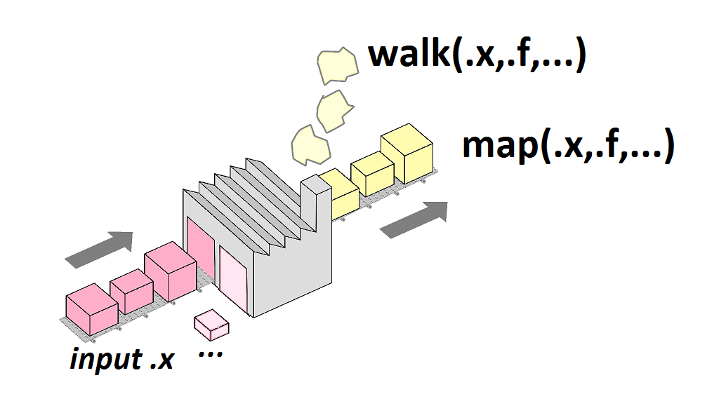
purrr
purrr is functional programming toolkit which enhances R with consistent tools for working with functions, lists and vectors.
Functional programming […] treats computation as the evaluation of mathematical functions and avoids changing-state and mutable data
— Wikipedia
An example function
Consider a hypothetic put_on() function


put_on(figures, antenna) returns a minifig with antenna
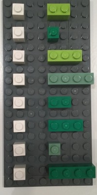
Figures LEGO pictures courtesy by Jennifer Bryan
Iteration with LEGO figures
Illustration for several lego
How to apply put_on() to more than 1 input?

put_on(figures, antenna)

Functional programming
Back to R programming
For loop approach
Of course, someone has to write loops. It doesn’t have to be you.
— Jenny Bryan
Your turn
10:00
Questions
Calculate the median for all columns in the trees data set, packaged with R.
You should be able to find three solutions,
- one returning a list,
- a vector of doubles and
- a tibble with a single row respectively.
Tips
purrr::map()expects 2 arguments:- a
list - a
function
- a
- A
data.frameis a list - Each column represents an element of the list i.e. a data frame is a list of vectors
Answer
The for loop machinery
means <- vector("list", ncol(swiss))
for (i in seq_along(swiss)) {
  means[i] <- mean(swiss[[i]])
}
# Need to manually add names
names(means) <- names(swiss)
means |>
  str()
List of 6
$ Fertility : num 70.1
$ Agriculture : num 50.7
$ Examination : num 16.5
$ Education : num 11
$ Catholic : num 41.1
$ Infant.Mortality: num 19.9Better answer
Functional programming focuses on actions
The purrr::map() family of functions
- Are designed to be consistent
map(),map2()andpmap()return a lists
- Typed variants with vectorized output:
map_lgl()map_int()map_dbl()map_chr()map_dfr()data.frame rowsmap_dfc()data.frame cols
- Fail if coercion is impossible
       Fertility      Agriculture      Examination        Education
        70.14255         50.65957         16.48936         10.97872
        Catholic Infant.Mortality
41.14383 19.94255 Fertility Agriculture Examination Education
"70.142553" "50.659574" "16.489362" "10.978723"
Catholic Infant.Mortality
"41.143830" "19.942553" Error in `map_int()`:
ℹ In index: 1.
ℹ With name: Fertility.
Caused by error:
! Can't coerce from a number to an integer.Adapted from the tutorial of Jennifer Bryan
purrr and base R
apply() family of functions
map()is the general function and close tobase::lapply()- Both return lists
map_dbl()generating vectors are similar tosapply()map()introduces shortcuts- Generally easier to use and more consistent
- Similar in idea to
map()in Python
apply(),tapply()andvapply()have varying return types and are best avoided even when using pure base R.
Examples
       Fertility      Agriculture      Examination        Education
        70.14255         50.65957         16.48936         10.97872
        Catholic Infant.Mortality
41.14383 19.94255 $Fertility
[1] 70.14255
$Agriculture
[1] 50.65957
$Examination
[1] 16.48936
$Education
[1] 10.97872
$Catholic
[1] 41.14383
$Infant.Mortality
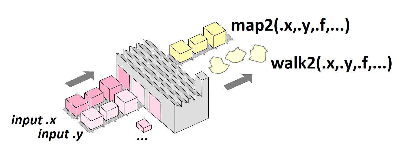
[1] 19.94255Iterating on 2 lists in parallel


Practical examples
map2()
marks <- list(report = c(14, 13),
              practical = c(10, 12),
              theoretical = c(17, 8))

weights <- c(2, 0.5, 1.5)

map2(marks, weights,  \(x, y) x * y)
$report
[1] 28 26
$practical
[1] 5 6
$theoretical
[1] 25.5 12.0Iterate on list (marks), but vectorized on atomic vectors (weights).
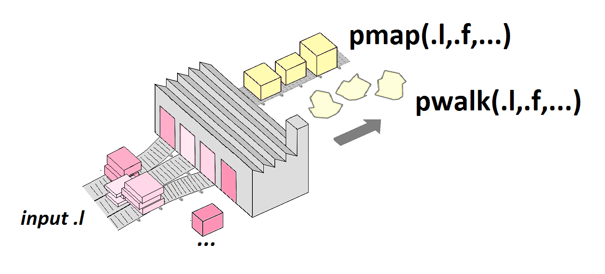
pmap()
Generate grid of values for named arguments of a function
Linear modelling
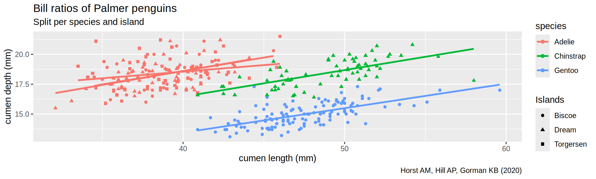
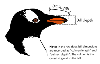
Palmer penguins
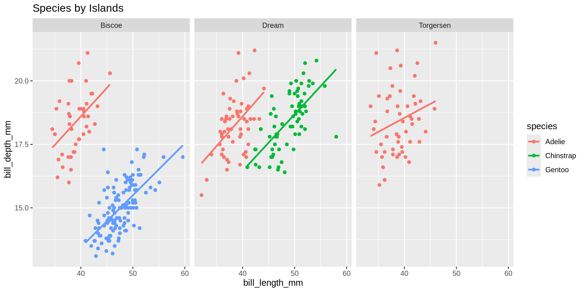
palmerpenguins from Horst AM, Hill AP, Gorman KB (2020)
Fitting a linear model
Using the pinguins dataset we can fit a linear model to explain the bill depth by the bill_length_mm.
lm outputs complex lists
Call:
lm(formula = bill_depth_mm ~ bill_length_mm, data = penguins)

Residuals:
    Min      1Q  Median      3Q     Max
-4.1381 -1.4263  0.0164  1.3841  4.5255

Coefficients:
               Estimate Std. Error t value Pr(>|t|)
(Intercept)    20.88547    0.84388  24.749  < 2e-16 ***
bill_length_mm -0.08502    0.01907  -4.459 1.12e-05 ***
---
Signif. codes:  0 '***' 0.001 '**' 0.01 '*' 0.05 '.' 0.1 ' ' 1

Residual standard error: 1.922 on 340 degrees of freedom
  (2 observations deleted due to missingness)
Multiple R-squared:  0.05525,   Adjusted R-squared:  0.05247
F-statistic: 19.88 on 1 and 340 DF,  p-value: 1.12e-05
Summarise a linear model with
base::summary()
- \(R^2\) is low (
0.05525) because we mix all individuals. - We need one tibble per group
Split the penguin data
Split a data.frame by group into a list of tibble
Get the dimensions of each tibble in the list
Map the linear model
General syntax: map(list, function)
listsplit_pengfunctioncan be an anonymous function
Curly braces are optional but helpful
- Several code lines
- Wrap lines to improve readability
[[1]]

Call:
lm(formula = bill_depth_mm ~ bill_length_mm, data = x)

Coefficients:
   (Intercept)  bill_length_mm
        9.6263          0.2244


[[2]]

Call:
lm(formula = bill_depth_mm ~ bill_length_mm, data = x)

Coefficients:
   (Intercept)  bill_length_mm
        5.2510          0.2048


[[3]]

Call:
lm(formula = bill_depth_mm ~ bill_length_mm, data = x)

Coefficients:
   (Intercept)  bill_length_mm
        9.2607          0.2335


[[4]]

Call:
lm(formula = bill_depth_mm ~ bill_length_mm, data = x)

Coefficients:
   (Intercept)  bill_length_mm
        7.5691          0.2222


[[5]]

Call:
lm(formula = bill_depth_mm ~ bill_length_mm, data = x)

Coefficients:
   (Intercept)  bill_length_mm
       14.1359          0.1102
To extract \(R^2\)
base::summary() generates a list
lm_all <- summary(lm(bill_depth_mm ~ bill_length_mm,
                     data = penguins))
str(lm_all, max.level = 1, give.attr = FALSE)
List of 12
$ call : language lm(formula = bill_depth_mm ~ bill_length_mm, data = penguins)
$ terms :Classes 'terms', 'formula' language bill_depth_mm ~ bill_length_mm
$ residuals : Named num [1:342] 1.139 -0.127 0.541 1.535 3.056 ...
$ coefficients : num [1:2, 1:4] 20.8855 -0.085 0.8439 0.0191 24.7492 ...
$ aliased : Named logi [1:2] FALSE FALSE
$ sigma : num 1.92
$ df : int [1:3] 2 340 2
$ r.squared : num 0.0552
$ adj.r.squared: num 0.0525
$ fstatistic : Named num [1:3] 19.9 1 340
$ cov.unscaled : num [1:2, 1:2] 1.93e-01 -4.32e-03 -4.32e-03 9.84e-05
$ na.action : 'omit' Named int [1:2] 4 272Extract \(R^2\) for all groups
Using anonymous functions
Further simplifications
With shortcuts from purrr
With coercion to doubles vector map_dbl()
split_peng |>
  map(\(x) lm(bill_depth_mm ~ bill_length_mm,
              data = x)) |>
  map(summary) |>
  map_dbl("r.squared")
[1] 0.21920517 0.41394290 0.25792423 0.42710958 0.06198376purrr anonmyous functions
- The package contains its own lambda, which predates the
\()syntax in base R. - It uses
~in place of\()and has default placeholders starting with.. - We’re not going to use it.
Your turn
ChickWeight is an in-built data set relating the growth of chicken on a diet.
Which diet has the biggest increase in growth as expressed in weight over time?
- Split the chicken by diet using
group_split() - Build linear model with the
lmfunction. - Retrieve the model details with
summary(). - Extract the “coefficients” of the linear model which is a Matrix including a “time” row and a “Estimate” column.
15:00
Lists as a column in a tibble
Example
Picture by Jennifer Bryan
tibble(numbers = 1:8,
       my_list = list(a = c("a", "b"), b = 2.56,
                      c = c("a", "b", "c"), d = rep(TRUE, 4),
                      d = 2:3, e = 4:6, f = FALSE, g = c(1, 4, 5, 6)))
# A tibble: 8 × 2
numbers my_list
<int> <named list>
1 1 <chr [2]>
2 2 <dbl [1]>
3 3 <chr [3]>
4 4 <lgl [4]>
5 5 <int [2]>
6 6 <int [3]>
7 7 <lgl [1]>
8 8 <dbl [4]> Nesting
Rewriting our previous example
Nesting the tibble by island and species
Rewriting our previous example
With modelling using mutate and map
- Very powerful
- Data rectangle
- Next lecture will show you how
dplyr,tidyr,tibble,purrrandbroomnicely work together
# A tibble: 5 × 6
  island    species   data     model  summary
  <fct>     <fct>     <list>   <list> <list>
1 Torgersen Adelie    <tibble> <lm>   <smmry.lm>
2 Biscoe    Adelie    <tibble> <lm>   <smmry.lm>
3 Dream     Adelie    <tibble> <lm>   <smmry.lm>
4 Biscoe    Gentoo    <tibble> <lm>   <smmry.lm>
5 Dream     Chinstrap <tibble> <lm>   <smmry.lm>
# ℹ 1 more variable: r_squared <dbl>
Don’t forget vectorisation!
Don’t “overmap” functions!
- Use
map()only if required for functions that are not vectorised.
Calling a function for its side-effects
Side effects are not pure
- Output on screen
- Save files to disk
- The return values are not used for further list-wise computation.
The map family should not be used.
Use the walk family of function
walk(),walk2()- Returns the input list (invisibly)
Saving 5 plots using indices for filenames
iwalk(split_peng,  \(x, y) {
  ggplot(x, aes(x = island)) +
    geom_bar() +
    # extract vector then unique species string
    labs(title = pull(x, species) |>
                   str_unique())
    ggsave(glue::glue("{y}_peng.pdf"))
})

fs::dir_ls(glob = "*_peng.pdf")
1_peng.pdf 2_peng.pdf 3_peng.pdf 4_peng.pdf 5_peng.pdf 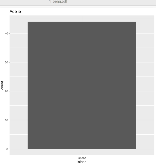
Wrap up
Assignment and environments
Other assignment operators
<- Left assignment operator
Most commonly used.
Rstudio has the built-in shortcut Alt+- for <-.
-> Right assignment operator
Right assignment in long pipe statements
swiss |>
  as_tibble(rownames = "Province") |>
  mutate(First = str_extract(Province, "^.")) |>
  group_by(First) |>
  summarize(across(where(is.numeric),
                   mean)) -> swiss_province_group

swiss_province_group
# A tibble: 17 × 7
First Fertility Agriculture Examination
<chr> <dbl> <dbl> <dbl>
1 A 66.6 63.4 18
2 B 77.1 54.3 21
3 C 72.5 57.4 13.3
4 D 83.1 45.1 6
5 E 68.8 78.8 12.5
6 F 92.5 39.7 5
7 G 82.2 51.7 14.3
8 H 77.3 89.7 5
9 L 62.7 26.4 25.4
10 M 73.2 58.9 13.4
11 N 66.0 37.3 24.7
12 O 65.0 62.6 16
13 P 74.1 52.3 9.67
14 R 49.3 45.0 18
15 S 79.8 67.2 10.2
16 V 65.1 29.8 23.2
17 Y 65.4 49.5 15
# ℹ 3 more variables: Education <dbl>,
# Catholic <dbl>, Infant.Mortality <dbl>The case of the equal sign
= Named parameter operator
Double meaning of =
- Alias of left assignment
<-. - Parameter - argument operator
Parental assignment
Parental assignment operators
Left <<- and
Right ->>
Work as -> and <- but assign in Global Environment.
Breaking values out of pipes
::::
Use of parental assignment operators for side effects
Multiple filtering steps
swiss_tbl |>
  filter(Agriculture > 40) |>
  # how many rows?
  filter(Education   < 50) |>
  # how many rows?
  filter(Examination < 10)
# A tibble: 8 × 7
Province Fertility Agriculture Examination
<chr> <dbl> <dbl> <int>
1 Delemont 83.1 45.1 6
2 Paysd'enhaut 72 63.5 6
3 Conthey 75.5 85.9 3
4 Entremont 69.3 84.9 7
5 Herens 77.3 89.7 5
6 Monthey 79.4 64.9 7
7 St Maurice 65 75.9 9
8 Sierre 92.2 84.6 3
# ℹ 3 more variables: Education <int>,
# Catholic <dbl>, Infant.Mortality <dbl>Better counter function
counter_name <- function(df, n_name){
  assign(n_name, nrow(df))
  df
}
counter_name(swiss_tbl, "n_filter_1" )
# A tibble: 47 × 7
Province Fertility Agriculture Examination
<chr> <dbl> <dbl> <int>
1 Courtelary 80.2 17 15
2 Delemont 83.1 45.1 6
3 Franches-Mnt 92.5 39.7 5
4 Moutier 85.8 36.5 12
5 Neuveville 76.9 43.5 17
6 Porrentruy 76.1 35.3 9
7 Broye 83.8 70.2 16
8 Glane 92.4 67.8 14
9 Gruyere 82.4 53.3 12
10 Sarine 82.9 45.2 16
# ℹ 37 more rows
# ℹ 3 more variables: Education <int>,
# Catholic <dbl>, Infant.Mortality <dbl>Error: object 'n_filter_1' not foundFinal options
Global name space pollution
Before we stop
You learned to
- Functional programming: focus on
actions forloops are fine, but don’t write them- Pass
functionsasarguments - Apprehend nested tibbles with
list-columns
Acknowledgments
- Eric Koncina for writing the initial content
- Jennifer Bryan (LEGO pictures, courtesy CC licence)
- Hadley Wickham
- Lise Vaudor
- Ian Lyttle
- Jim Hester
Further reading
- Jennifer Bryan - lessons & tutorial
- Hadley Wickham - R for data science (iteration, many models)
- Ian Lyttle - purrr applied for engineering
- Robert Rudis - purrr, comparison with base
- Rstudio’s blog - purrr 0.2 release purrr 0.3 release
- Kris Jenkins - What is Functional Programming? (Blog version and Talk video)
- Lise Vaudor - R-atique (in french)
Thank you for your attention!
![]()